Bayesian Optimization in Chemical Synthesis: Accelerating Drug Discovery with AI
This article explores the transformative role of Bayesian Optimization (BO) in efficiently identifying optimal chemical reaction conditions, a critical and resource-intensive challenge in pharmaceutical development.
Bayesian Optimization in Chemical Synthesis: Accelerating Drug Discovery with AI
Abstract
This article explores the transformative role of Bayesian Optimization (BO) in efficiently identifying optimal chemical reaction conditions, a critical and resource-intensive challenge in pharmaceutical development. It covers the foundational principles of BO, including Gaussian Process surrogate models and acquisition functions that balance exploration and exploitation. The scope extends to practical methodologies and applications in high-throughput experimentation (HTE), troubleshooting common pitfalls, and validating performance against traditional approaches. Through case studies and comparative analysis, we demonstrate how BO enables rapid optimization of complex reactions, such as Suzuki and Buchwald-Hartwig couplings, significantly shortening process development timelines for Active Pharmaceutical Ingredients (APIs) and paving the way for autonomous laboratories.
What is Bayesian Optimization? Core Principles Transforming Chemical Reaction Screening
The Challenge of Chemical Reaction Optimization in Pharmaceutical Development
Troubleshooting Guide: Bayesian Optimization in Action
This guide addresses common challenges scientists face when implementing Bayesian Optimization (BO) for chemical reaction optimization in pharmaceutical development.
FAQ 1: My Bayesian optimization algorithm suggests experiments that seem theoretically impossible to improve yield. Why does this happen, and how can I prevent it?
- Problem: Standard BO algorithms can sometimes suggest experimental conditions that are "futile" – meaning that even with a 100% yield, they could not improve the current best objective value, especially when optimizing complex functions like throughput.
- Solution: Implement an Adaptive Boundary Constraint (ABC-BO) strategy. This method incorporates knowledge of the objective function into the BO process. It dynamically identifies and excludes futile experimental conditions as the optimization progresses, allowing the algorithm to focus only on the most promising regions of the search space. This has been shown to prevent up to 50% of futile experiments in complex optimizations involving multiple categorical, continuous, and discrete variables [1].
- Recommended Action: Review your objective function and integrate a check that assesses whether a suggested condition has the theoretical potential to surpass the current best value before running the experiment.
FAQ 2: How can I effectively explore a vast condition space with many categorical variables (like ligands and solvents) without exhaustive screening?
- Problem: The high dimensionality of reaction condition spaces, particularly with categorical variables, makes exhaustive screening intractable, even with High-Throughput Experimentation (HTE).
- Solution: Use a scalable BO framework (e.g., Minerva) designed for large parallel batches and high-dimensional spaces. The workflow should start with algorithmic quasi-random sampling (e.g., Sobol sampling) to diversify initial space coverage. Subsequently, an acquisition function guided by a surrogate model (like a Gaussian Process) balances the exploration of unknown regions with the exploitation of known promising conditions [2].
- Recommended Action: Frame your reaction space as a discrete combinatorial set of plausible conditions, automatically filtering out impractical combinations (e.g., temperatures exceeding solvent boiling points). This allows the BO algorithm to efficiently navigate spaces with tens of thousands of potential conditions [2].
FAQ 3: My experimental results are noisy. Is Bayesian optimization still suitable?
- Problem: Chemical reaction data often contains inherent noise and variability, which can derail optimization algorithms.
- Solution: Yes, BO is suitable. Its probabilistic nature, through surrogate models like Gaussian Processes, inherently handles uncertainty. The algorithm uses prediction uncertainty to guide experimentation, making it robust to noisy data. Furthermore, noise-robust methods and multi-task learning are emerging techniques that enhance BO's versatility in such scenarios [2] [3].
- Recommended Action: Ensure your BO implementation uses a surrogate model and acquisition functions that explicitly account for noise. Techniques such as Noisy Expected Hypervolume Improvement (q-NEHVI) are designed for such environments [2] [3].
FAQ 4: Bayesian optimization feels like a "black box." How can I understand why it suggests certain conditions?
- Problem: The decision-making process of sophisticated BO models can be opaque, making it difficult for chemists to trust, validate, or align suggestions with their expertise.
- Solution: Consider alternative, more interpretable optimization frameworks. Swarm Intelligence approaches, such as the α-PSO algorithm, offer a solution. α-PSO uses mechanistically clear, physics-inspired swarm dynamics where the movement of "particles" (representing experiments) is guided by simple rules based on personal best, swarm best, and a machine learning term. This provides a transparent view of the factors driving each optimization decision [4].
- Recommended Action: For critical projects where interpretability is key, explore hybrid metaheuristic algorithms like α-PSO, which have demonstrated performance competitive with state-of-the-art BO while maintaining methodological clarity [4].
Performance Data: Bayesian Optimization in Pharmaceutical Research
The table below summarizes quantitative data from real-world applications of Bayesian optimization in pharmaceutical development.
Table 1: Performance Metrics of Bayesian Optimization in Pharmaceutical Reaction Optimization
| Application Context | Optimization Target | Key Performance Outcome | Experimental Efficiency | Source |
|---|---|---|---|---|
| Ni-catalyzed Suzuki & Pd-catalyzed Buchwald-Hartwig API syntheses | Yield & Selectivity | Identified multiple conditions achieving >95% area percent yield and selectivity | Led to improved process conditions at scale in 4 weeks vs. a previous 6-month campaign [2] | |
| General catalytic reaction optimization | Finding optimal conditions | Found optimal conditions in 4 rounds of 10 experiments from a pool of 180,000 possibilities | Tested just <0.02% of total possibilities, representing an estimated 85% reduction in experiments [5] | |
| Algorithmic Process Optimization (APO) with Merck | Multi-objective problems at scale | Awarded 2025 ACS Green Chemistry Award for sustainable innovation | Reduced hazardous reagents, material waste, and accelerated development timelines [6] |
Experimental Protocols: Key Bayesian Optimization Workflows
Protocol 1: Scalable Multi-Objective Optimization with Minerva
This methodology is designed for highly parallel HTE campaigns, such as in 96-well plates [2].
- Problem Formulation: Define the reaction condition space as a discrete combinatorial set of plausible conditions, incorporating practical constraints (e.g., solvent safety, boiling points).
- Initial Sampling: Use quasi-random Sobol sampling to select an initial batch of experiments. This maximizes initial coverage of the reaction space.
- Model Training & Experiment Selection:
- Train a Gaussian Process (GP) regressor on the collected experimental data to predict reaction outcomes (e.g., yield, selectivity) and their uncertainties.
- Use a scalable multi-objective acquisition function (e.g., q-NParEgo, TS-HVI, or q-NEHVI) to evaluate all possible conditions and select the next batch of experiments. This function balances exploring uncertain regions and exploiting known high-performing areas.
- Iteration: Repeat the cycle of experimentation, model updating, and batch selection until objectives are met or the experimental budget is exhausted.
Protocol 2: Adaptive Boundary Constraint Bayesian Optimization (ABC-BO)
This protocol is designed to prevent futile experiments in complex reaction spaces [1].
- Standard BO Setup: Begin a standard Bayesian optimization process with a defined objective function and search space.
- Boundary Assessment: Before executing a suggested experiment, calculate whether the given conditions could theoretically improve the existing best objective, even assuming a 100% yield.
- Constraint Application: If the experiment is deemed "futile," the algorithm adaptively excludes it and re-directs the acquisition function to suggest a more promising condition.
- Focused Optimization: As the optimization progresses, the algorithm dynamically narrows its focus to the shrinking set of truly promising experimental conditions, maximizing the value of each experiment.
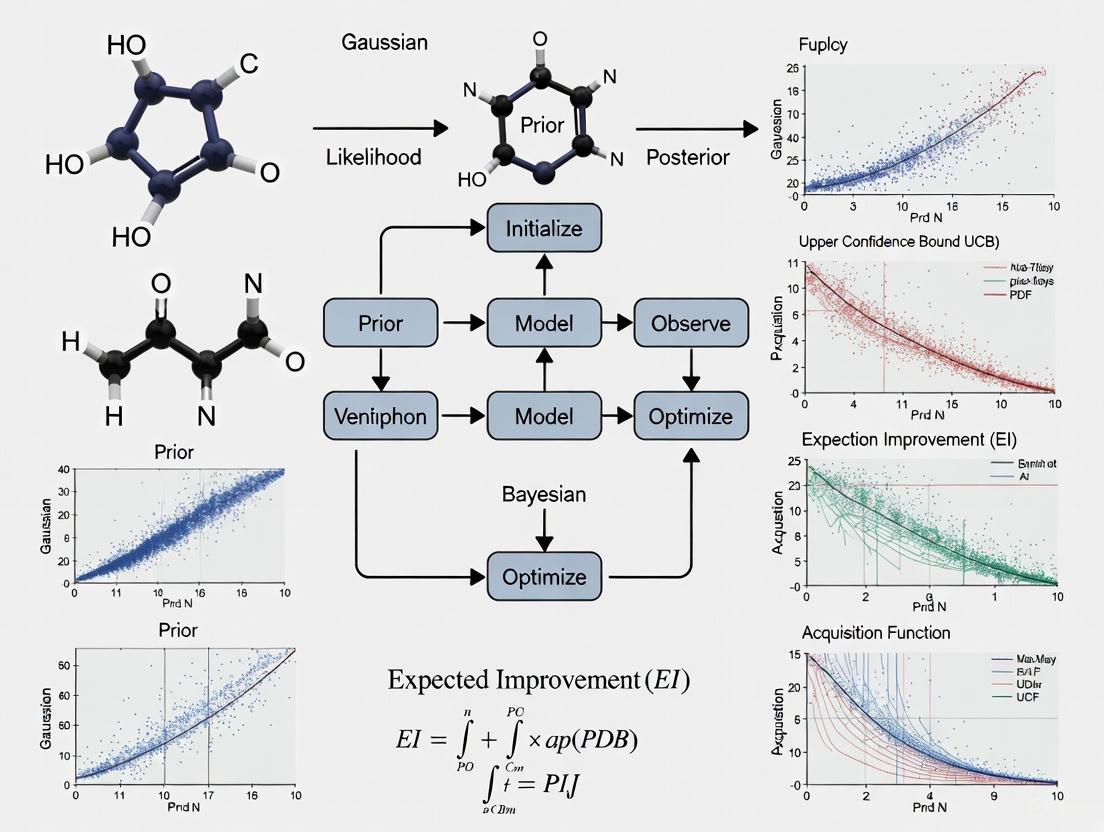
Workflow Visualization: Bayesian Optimization Logic
The diagram below illustrates the core iterative workflow of a Bayesian Optimization campaign for chemical reaction development.
Core Bayesian Optimization Workflow
The Scientist's Toolkit: Research Reagent Solutions
The table below lists key materials and their functions in machine-learning-driven reaction optimization campaigns, as featured in the cited research.
Table 2: Essential Research Reagents and Their Functions in ML-Driven Optimization
| Reagent / Material | Function in Optimization | Example Context |
|---|---|---|
| Nickel Catalysts | Earth-abundant, cost-effective alternative to precious metal catalysts for cross-coupling reactions. | Ni-catalyzed Suzuki reaction optimization [2] [4] |
| Palladium Catalysts | High-performance catalysts for key C-C and C-N bond-forming reactions like Suzuki and Buchwald-Hartwig couplings. | Pd-catalyzed Buchwald-Hartwig amination [2] [4] |
| Ligand Libraries | Modular components that significantly influence catalyst activity and selectivity; a primary categorical variable for screening. | Explored in high-dimensional search spaces to find optimal catalyst systems [2] |
| Solvent Sets | Medium that affects reaction kinetics, solubility, and mechanism; a key categorical variable to optimize. | Screened following pharmaceutical green chemistry guidelines (e.g., solvent selection guides) [2] |
| High-Throughput Experimentation (HTE) Platforms | Automated robotic systems enabling miniaturized, highly parallel execution of reactions (e.g., in 96-well plates). | Essential for generating the large datasets required for efficient ML-guided optimization [2] [4] |
| Chitin synthase inhibitor 8 | Chitin synthase inhibitor 8, MF:C23H23N3O5, MW:421.4 g/mol | Chemical Reagent |
| 3-epi-Azido-3-deoxythymidine | 3-epi-Azido-3-deoxythymidine, MF:C10H13N5O4, MW:267.24 g/mol | Chemical Reagent |
Bayesian Optimization as a Solution for Black-Box, Expensive-to-Evaluate Functions
Troubleshooting Guides and FAQs
Frequently Asked Questions
Q1: My Bayesian Optimization (BO) process is converging slowly. How can I improve its performance?
Slow convergence often stems from an imbalance between exploration and exploitation. You can adjust the acquisition function's parameters to better suit your problem. For the Expected Improvement (EI) function, increase the ξ (xi) parameter to encourage more exploration of uncertain regions [7] [8]. Additionally, ensure your initial dataset is sufficient; starting with too few random samples (e.g., less than 5-10) can lead to poor surrogate model fitting [9]. For high-dimensional spaces, consider using a Sobol sequence for initial sampling to maximize space-filling properties [2].
Q2: How should I handle categorical variables, like solvent or catalyst type, in my BO setup? Categorical variables require special treatment as standard Gaussian Processes (GPs) model continuous spaces. One effective approach is to represent the reaction condition space as a discrete combinatorial set of potential conditions [2]. Convert categorical parameters into numerical descriptors. The algorithm can then automatically filter out impractical combinations based on domain knowledge (e.g., excluding temperatures exceeding a solvent's boiling point) [2]. For ligand or solvent screening, treat each unique combination as a distinct category within the optimization space.
Q3: A significant portion of my experiments are "futile" – they cannot possibly improve the objective. How can I prevent this? Implement an Adaptive Boundary Constraint (ABC-BO) strategy [1]. Before running an experiment, check if the proposed conditions could theoretically improve the best-known objective, even assuming a 100% yield. If not, the algorithm should reject these conditions and propose new ones. This is particularly useful for objective functions like throughput, where physical limits can be calculated. This method has been shown to reduce futile experiments by up to 50% in complex reaction optimizations [1].
Q4: What should I do when my objective function evaluations are noisy or my measurements have significant experimental error? Incorporate a nugget term (also known as a jitter term) into your Gaussian Process model [9]. This term, added to the diagonal of the covariance matrix, accounts for measurement noise and improves computational stability. Estimate the noise level from your data if possible, or set it to a small positive value. Using a nugget is recommended even for deterministic simulations, as it helps account for the bias between the simulation and reality [9].
Q5: How can I optimize for multiple objectives simultaneously, such as maximizing yield while minimizing cost? Use Multi-Objective Bayesian Optimization (MOBO). For highly parallel setups (e.g., 96-well plates), scalable acquisition functions like q-NParEgo, Thompson Sampling with Hypervolume Improvement (TS-HVI), or q-Noisy Expected Hypervolume Improvement (q-NEHVI) are recommended [2]. These functions efficiently handle multiple competing objectives and large batch sizes. Performance can be evaluated using the hypervolume metric, which measures both convergence towards optimal objectives and the diversity of solutions [2].
Troubleshooting Common Experimental Issues
Problem: The algorithm seems stuck in a local optimum.
- Potential Cause: Over-exploitation due to an acquisition function that favors known high-performing regions too heavily.
- Solution: Switch to the "plus" variant of your acquisition function (e.g.,
expected-improvement-plus), which detects overexploitation and modifies the kernel function to increase variance in unexplored areas, encouraging escape from local optima [10]. Alternatively, manually increase the exploration parameter in EI or UCB functions.
Problem: The Gaussian Process model is taking too long to fit.
- Potential Cause: The computational complexity of GPs scales as O(N³) with the number of data points, becoming slow with hundreds of evaluations [11].
- Solution: For problems requiring many evaluations, consider surrogate models that scale better, such as Random Forests or Bayesian Neural Networks [3]. Since experimental evaluations are expensive, staying below 1000 data points is common, where GPs remain manageable [11].
Problem: BO fails to find good conditions in a very large search space.
- Potential Cause: The search space is too vast or contains many impractical regions.
- Solution: Integrate domain expertise to define a plausible reaction condition space first [2]. Use algorithmic quasi-random sampling (e.g., Sobol sequences) for the initial batch to ensure broad coverage. This increases the likelihood of discovering informative regions containing global optima.
Bayesian Optimization Components and Performance
Table 1: Common Acquisition Functions and Their Use Cases
| Acquisition Function | Key Characteristics | Best For |
|---|---|---|
| Expected Improvement (EI) [7] [10] | Balances probability and amount of improvement; most widely used [8]. | General-purpose optimization; a reliable default choice. |
| Probability of Improvement (PI) [7] [10] | Focuses on the likelihood of improvement, can get stuck in local optima. | When a quick, simple solution is needed; less recommended for global optimization. |
| Upper Confidence Bound (UCB) [10] [9] | Uses a confidence bound parameter (κ) to explicitly balance exploration and exploitation. | Problems where a clear trade-off between exploration/exploitation is desired. |
| q-Noisy Expected Hypervolume Improvement (q-NEHVI) [2] | Scalable, multi-objective acquisition function. | Simultaneous optimization of multiple objectives (e.g., yield, cost, selectivity) in large batches. |
| Thompson Sampling (TS) [2] [3] | Randomly draws functions from the posterior and selects the best point. | Multi-objective optimization and highly parallel batch evaluations. |
Table 2: Key Reagent Solutions for a Bayesian Optimization Campaign
| Reagent / Component | Function in the Optimization |
|---|---|
| Gaussian Process (GP) [7] [9] | Core surrogate model; approximates the unknown objective function and provides uncertainty estimates. |
| Matérn 5/2 Kernel [10] [9] | A common covariance function for the GP; less smooth than the RBF kernel, making it better for modeling physical phenomena [9]. |
| Nugget Term [9] | A small value added to the kernel's diagonal to account for experimental noise and improve numerical stability. |
| Sobol Sequence [2] | A quasi-random sequence for selecting initial experiments; ensures the design space is evenly sampled. |
| Hypervolume Metric [2] | A performance metric for multi-objective optimization; calculates the volume of objective space dominated by the found solutions. |
Experimental Protocol: A Standard Bayesian Optimization Workflow
The following workflow is adapted from real-world applications in chemical synthesis [2] [3].
Problem Definition
- Define the objective(s) (e.g., reaction yield, selectivity, space-time yield).
- Identify all optimization variables (continuous: temperature, concentration; categorical: solvent, catalyst).
- Set feasible bounds for all variables.
Initial Experimental Design
- Select an initial set of experiments using a Sobol sequence or random sampling within the defined bounds.
- For a typical 96-well HTE plate, a common initial batch size is 24, 48, or 96 reactions [2].
- Run the experiments and record the outcomes.
Model Fitting and Iteration
- Surrogate Model Construction: Fit a Gaussian Process model to the collected data. The Matern 5/2 kernel is often recommended [9].
- Hyperparameter Tuning: Optimize the GP's hyperparameters (length scales, output scale, noise variance) using Maximum Likelihood Estimation (MLE) [9].
- Next Experiment Selection: Use an acquisition function (e.g., EI) to determine the most promising conditions for the next batch of experiments.
- Automated Filtering: Apply constraints (like ABC-BO) to filter out futile experiments before execution [1].
- Data Augmentation: Run the new experiments and add the results to the dataset.
Termination
- Repeat Step 3 until a convergence criterion is met (e.g., no significant improvement over several iterations, a desired performance threshold is reached, or the experimental budget is exhausted).
Workflow and Algorithm Visualization
Troubleshooting Guide: Common Issues and Solutions
| Problem Category | Specific Symptom | Likely Cause | Recommended Solution | Key References |
|---|---|---|---|---|
| Surrogate Model | Poor model fit, inaccurate predictions in unexplored regions. | Incorrect prior width or over-smoothing due to improper kernel lengthscale. | Tune GP hyperparameters (amplitude, lengthscale) via Maximum Likelihood Estimation. Consider a more flexible kernel (e.g., Matern 5/2). | [12] [13] |
| Acquisition Function | Optimization gets stuck in local optima, lacks exploration. | Inadequate balance between exploration and exploitation (e.g., incorrect ϵ in PI, low β in UCB). |
Switch to a more robust AF like Expected Improvement (EI). For multi-objective problems, use q-NParEgo or TS-HVI. | [12] [7] [13] |
| Computational Performance | Long delays in selecting new experiments, especially with large batches. | High complexity of multi-objective acquisition functions (e.g., q-EHVI) scaling poorly with batch size. | Use scalable AFs like TS-HVI or q-NParEgo for large parallel batches (e.g., 96-well plates). | [2] |
| Prior Specification | Posterior results are biased or unrealistic. | Poorly chosen prior distributions that do not accurately reflect domain knowledge. | Perform sensitivity analysis on priors. Use hierarchical modeling or empirical Bayes to estimate priors from data. | [14] |
Frequently Asked Questions (FAQs)
What is the most suitable surrogate model for handling the noise commonly found in chemical reaction data?
Gaussian Processes (GPs) are the most commonly used and recommended surrogate model for Bayesian optimization in chemistry [15] [3] [13]. They are particularly effective because they not only provide a prediction (the posterior mean) but also a quantitative measure of uncertainty (the posterior variance) for any point in the search space [13]. This uncertainty quantification is crucial for guiding the exploration-exploitation trade-off. GPs can naturally handle noisy observations by incorporating a noise term (e.g., Gaussian noise) directly into the model [13].
How do I choose an acquisition function for simultaneously optimizing both reaction yield and selectivity?
When moving from a single objective to multiple objectives, you must use a multi-objective acquisition function. The core goal shifts from finding a single best point to mapping a Pareto front—a set of conditions where one objective cannot be improved without worsening another [2] [3].
For highly parallel experimentation, such as 96-well HTE plates, traditional methods like q-EHVI can be computationally slow. In these cases, it is recommended to use more scalable functions like:
- q-NParEgo
- Thompson Sampling with Hypervolume Improvement (TS-HVI) [2]
These functions are designed to efficiently handle large batch sizes and high-dimensional search spaces common in real-world laboratories [2].
Our optimization keeps converging to a local optimum. How can we encourage more exploration?
This is a classic sign of an acquisition function that is over-exploiting. You can address this by:
- Adjusting AF Parameters: If using Probability of Improvement (PI), increase the
ϵparameter to encourage exploring more uncertain regions. If using Upper Confidence Bound (UCB), increase theβparameter to give more weight to the uncertainty term [7]. - Switching the AF: Consider using Expected Improvement (EI), which typically offers a better balance by considering both the probability and magnitude of improvement [15] [13]. It is a popular choice due to its well-balanced performance and straightforward analytic form [15].
What are the best practices for specifying priors in the Gaussian Process model when historical data is limited?
Specifying priors is a known challenge in Bayesian methods [14]. With limited data, you can:
- Use Sensitivity Analysis: Test how different prior choices affect your final results to ensure they are not introducing bias [14].
- Adopt Hierarchical Modeling: This allows you to incorporate multiple levels of information, making the model more robust [14].
- Leverage Chemical Intuition: Your domain knowledge as a chemist is invaluable. Use it to define reasonable bounds and constraints for the search space (e.g., excluding solvent and temperature combinations that would cause boiling) [2] [16].
The Scientist's Toolkit: Research Reagent Solutions
| Item | Function in Bayesian Optimization | Key Considerations |
|---|---|---|
| Gaussian Process (GP) | Serves as the core surrogate model; approximates the expensive black-box function (e.g., reaction yield) and provides uncertainty estimates. | The Matern 5/2 kernel is recommended for practical optimization due to its flexibility [13]. Hyperparameters (lengthscale, amplitude) must be tuned. |
| Expected Improvement (EI) | A popular acquisition function that selects the next experiment by calculating the expected value of improving upon the current best result. | Balances exploration and exploitation effectively and has an analytic form for efficient computation [15] [13]. |
| Sobol Sequence | A space-filling design algorithm used to select the initial set of experiments before the Bayesian loop begins. | Maximally spreads out initial experiments across the search space, increasing the chance of finding promising regions early [2]. |
| Thompson Sampling (TS-HVI) | A multi-objective acquisition function suitable for large parallel batches. Efficiently scales to 96-well plates. | Helps overcome the computational bottlenecks of other multi-objective functions like q-EHVI in high-throughput settings [2]. |
| 9-Dihydroestradiol-d3 | 9-Dihydroestradiol-d3, MF:C18H22O2, MW:273.4 g/mol | Chemical Reagent |
| Xanthine oxidase-IN-6 | Xanthine oxidase-IN-6, MF:C29H34N2O15, MW:650.6 g/mol | Chemical Reagent |
Experimental Protocol: A Standard Bayesian Optimization Workflow
The following diagram illustrates the iterative cycle of Bayesian Optimization, which can be applied to the optimization of chemical reactions.
Step-by-Step Methodology:
- Initial Design: Use a space-filling design like Sobol sampling to select an initial set of
nâ‚€reaction conditions (e.g., 10-20% of your experimental budget). This maximizes early information gain about the landscape [2] [13]. - Run Experiments: Conduct the chemical reactions at the chosen conditions and measure the outcomes (e.g., yield, selectivity, etc.).
- Update Dataset: Add the new {reaction conditions, results} pairs to your growing dataset
Dâ‚™. - Build Surrogate Model: Train a Gaussian Process (GP) model on the current dataset
Dâ‚™. The GP will model the objective function across the entire search space, providing predictions and uncertainty estimates [13]. - Maximize Acquisition Function: Using the trained GP, compute an acquisition function (AF) like Expected Improvement (EI) across the search space. Identify the reaction condition that maximizes this function [15] [13].
- Check Stopping Criterion: If the experimental budget is exhausted, a satisfactory result is found, or further iterations show no improvement, stop the process. Otherwise, return to Step 2 with the new candidate suggested by the AF.
Workflow Diagram: Multi-Objective Optimization with Large Batches
For industrial applications like pharmaceutical process development, optimization often involves multiple objectives and highly parallel experiments. The following diagram outlines a workflow adapted for this scale.
Key Adaptations for Scale:
- Condition Space: The search space is defined as a discrete set of plausible reaction conditions, automatically filtering out unsafe or impractical combinations (e.g., NaH in DMSO, temperatures exceeding solvent boiling points) [2].
- Scalable Acquisition: Instead of selecting one experiment per iteration, the AF selects a large batch of experiments in parallel. This requires using scalable AFs like TS-HVI or q-NParEgo that can handle the computational load of proposing dozens of experiments at once [2].
- Objective: The outcome is a set of Pareto-optimal conditions, giving process chemists multiple viable options that represent the best trade-offs between competing objectives like yield, selectivity, and cost [2].
Within the framework of a thesis on Bayesian optimization for chemical reaction conditions research, Gaussian Processes (GPs) serve as a cornerstone for building intelligent, data-efficient optimization systems. A GP is a probabilistic machine learning model that defines a distribution over functions, perfectly suited for approximating the complex, often non-linear relationship between reaction parameters (e.g., temperature, concentration, solvent choice) and experimental outcomes (e.g., yield, selectivity) [3]. In Bayesian optimization (BO), the GP acts as a surrogate model, or emulator, of the expensive-to-evaluate experimental function. It provides not just a prediction of the outcome for untested conditions but, crucially, a measure of uncertainty for that prediction [17] [18]. This uncertainty quantification is the engine of BO, enabling acquisition functions to strategically balance the exploration of unknown regions of the reaction space with the exploitation of known promising conditions, thereby accelerating the discovery of optimal reaction parameters with minimal experimental effort [3] [18].
Troubleshooting Guide: Common GP Challenges in Reaction Optimization
This guide addresses specific, high-impact challenges researchers may encounter when applying GPs to chemical reaction optimization.
Poor Model Performance and Prediction Inaccuracy
- Problem: GP predictions are inaccurate or the model is overconfident in incorrect predictions, leading to poor optimization guidance.
- Causes & Solutions:
- Inadequate Kernel Function: The kernel determines the GP's assumptions about the function's behavior. A standard Squared Exponential (Radial Basis Function) kernel assumes a very smooth response, which may not hold for complex chemical landscapes.
- Solution: Experiment with more flexible kernel structures. The Matérn kernel (e.g., Matérn 5/2) is a robust default as it accommodates less smooth functions [18]. For specialized applications, custom kernel combinations (e.g., additive or multiplicative kernels) can be tested to capture different scales of variation [19].
- Dominant Mean Function: An overly strong prior mean function can cause the model to ignore the data, leading to high confidence in poor predictions.
- Solution: Weaken the influence of the mean function, for example, by using a constant mean and optimizing its hyperparameter, rather than a complex, fixed mean function [20].
- Improperly Optimized Hyperparameters: The kernel's hyperparameters (e.g., length scale, noise) control the model's fit.
- Inadequate Kernel Function: The kernel determines the GP's assumptions about the function's behavior. A standard Squared Exponential (Radial Basis Function) kernel assumes a very smooth response, which may not hold for complex chemical landscapes.
Handling Categorical and High-Dimensional Inputs
- Problem: Reaction optimization involves categorical variables (e.g., solvents, ligands, catalysts) and potentially many continuous parameters, making standard GP application difficult.
- Causes & Solutions:
- Non-Numerical Inputs: Standard GP kernels operate on continuous numerical spaces.
- High-Dimensional Search Space: The computational cost of GPs scales poorly with the number of dimensions, and modeling becomes data-inefficient.
- Solution: Use dimension reduction techniques like Karhunen-Loève (KL) expansions to approximate the high-dimensional input field with a finite number of dominant stochastic dimensions, making emulation computationally feasible [17].
Managing Multiple Objectives and Outputs
- Problem: Chemical optimization typically involves multiple, often competing objectives (e.g., maximizing yield while minimizing cost or environmental impact). Standard single-task GPs cannot model correlations between these outputs.
- Causes & Solutions:
- Independent Modeling is Suboptimal: Modeling each property with an independent GP fails to leverage shared information, slowing down the discovery process.
- Solution: Employ multi-task GPs (MTGPs) or hierarchical models like Deep GPs (DGPs). These use advanced kernel structures to capture correlations between distinct material properties, allowing information from one objective to inform others and significantly accelerating multi-objective optimization [22].
- Independent Modeling is Suboptimal: Modeling each property with an independent GP fails to leverage shared information, slowing down the discovery process.
Computational Bottlenecks with Large Datasets
- Problem: GP training time becomes prohibitively slow as the number of experimental data points increases, hindering rapid iteration.
- Causes & Solutions:
- Cubic Scaling Cost: The computational complexity of standard GP inference is O(n³), where n is the number of data points.
- Solution: For large-scale High-Throughput Experimentation (HTE) campaigns, utilize scalable GP approximations. Sparse GPs or inducing point methods (e.g., implemented in libraries like GAUCHE) approximate the full model using a subset of "inducing points," reducing computational cost while maintaining performance [21] [18].
- Cubic Scaling Cost: The computational complexity of standard GP inference is O(n³), where n is the number of data points.
Dealing with Bifurcating Solutions or Multiple Equilibria
- Problem: In some physico-chemical processes, multiple stable equilibrium states (bifurcating solutions) can exist for the same input parameters. A single GP emulator will fail in such regions, as it expects a single output for a given input.
- Causes & Solutions:
- Non-Unique Outputs: The presence of a bifurcation point violates the fundamental assumption of a function.
- Solution: Implement a combined classification and regression approach. First, use a Gaussian process classifier to predict which branch or class the output belongs to for a given input. Then, build separate GP regressors for each class of solutions to model the output within that branch, enabling successful uncertainty analysis near bifurcation points [17].
- Non-Unique Outputs: The presence of a bifurcation point violates the fundamental assumption of a function.
Frequently Asked Questions (FAQs)
Q1: Why is a GP preferred over other surrogate models like Random Forests in Bayesian optimization for chemistry? A1: GPs are intrinsically probabilistic, providing principled uncertainty estimates (predictive variances) directly from the model structure. This native uncertainty quantification is essential for the acquisition function to effectively balance exploration and exploitation. While other models can be adapted, GPs are particularly well-suited for data-scarce scenarios common in experimental chemistry [3] [18].
Q2: My experimental measurements are noisy. How can the GP model account for this?
A2: GPs can explicitly model observation noise by including a noise term in the covariance function. This is typically a white noise kernel. During model training, the hyperparameter associated with this noise term (often called the alpha or noise level parameter) is optimized from the data, allowing the GP to distinguish between the underlying trend and the stochastic noise in your experimental measurements [19] [18].
Q3: What is a key advantage of using BO with GPs over traditional Design of Experiments (DoE)? A3: The primary advantage is adaptivity. Traditional DoE relies on a fixed, pre-determined experimental plan. In contrast, BO using GPs is a sequential, model-based process. Each experiment informs the selection of the next, allowing the campaign to dynamically focus on the most promising regions of the search space. This often leads to finding optimal conditions in fewer experiments, saving valuable time and resources [18].
Q4: Are there specific acquisition functions recommended for multi-objective optimization in high-throughput chemistry? A4: Yes, for highly parallel HTE campaigns with multiple objectives, scalable acquisition functions are crucial. While q-Expected Hypervolume Improvement (q-EHVI) is powerful, its computational cost can be high. Functions like q-NParEgo, Thompson Sampling with Hypervolume Improvement (TS-HVI), and q-Noisy Expected Hypervolume Improvement (q-NEHVI) have been developed and benchmarked to handle large batch sizes (e.g., 96-well plates) efficiently in multi-objective settings [2].
Q5: How can I prevent my optimization algorithm from suggesting futile experiments? A5: You can incorporate domain knowledge directly into the BO loop. The Adaptive Boundary Constraint BO (ABC-BO) strategy is one such method. It uses knowledge of the objective function (e.g., knowing that yield cannot exceed 100%) to screen out experimental conditions that are mathematically incapable of improving the objective, even under ideal outcomes, thus preventing wasted experimental effort [1].
Essential Workflows and Protocols
Core GP Workflow for Reaction Optimization
The following diagram illustrates the standard iterative workflow for using a Gaussian Process in Bayesian optimization for chemical reactions.
Protocol: Implementing a GP-Based Optimization Campaign
This protocol outlines the steps for a single iteration within the broader workflow, corresponding to the "Train GP Surrogate Model" and "Optimize Acquisition Function" steps in the diagram.
- Objective: To optimize a Ni-catalyzed Suzuki reaction for maximum yield and selectivity.
- Search Space: 88,000 possible conditions defined by categorical (ligand, solvent, base) and continuous (temperature, concentration) variables [2].
Step-by-Step Method:
Initialization and First Batch:
- Select an initial set of experimental conditions (e.g., 1x 96-well plate) using a space-filling algorithm like Sobol sampling to ensure broad coverage of the search space [2].
- Execute the reactions and measure outcomes (Yield, Selectivity).
Data Preprocessing:
- Clean the data and handle any missing values.
- Standardize continuous variables (e.g., temperature, concentration) to have zero mean and unit variance.
- Encode categorical variables (e.g., solvent, ligand) using numerical descriptors or one-hot encoding. For complex molecules, use learned representations from libraries like GAUCHE [21].
GP Model Training:
- Model Choice: Select a GP model with a Matérn 5/2 kernel for flexibility [18].
- Multi-objective Handling: For simultaneous yield/selectivity optimization, use a Multi-Task GP (MTGP) to capture correlations between the two objectives [22].
- Training: Optimize the GP hyperparameters (length scales, noise variance) by maximizing the log marginal likelihood using a conjugate gradient algorithm.
Suggesting New Experiments:
- Define an acquisition function. For multi-objective problems, use q-Noisy Expected Hypervolume Improvement (q-NEHVI) [2].
- Optimize the acquisition function over the entire search space to identify the single set or batch of conditions that promises the greatest improvement.
- Return these conditions to the experimentalist for the next iteration.
Workflow for Handling Bifurcating Solutions
For complex reaction landscapes with multiple possible equilibria, a modified workflow is required.
The Scientist's Toolkit: Research Reagent Solutions
The following table details key computational and experimental resources essential for implementing GP-based optimization.
| Item Name | Function/Benefit | Example Use-Case |
|---|---|---|
| GAUCHE Library [21] | A specialized Python library providing kernels for structured chemical data (graphs, strings) and GP tools for chemistry. | Modeling the effect of different molecular catalysts or solvents on reaction yield. |
| Multi-Task GP (MTGP) [22] | A GP variant that learns correlations between multiple output properties (e.g., yield & selectivity), accelerating multi-objective optimization. | Simultaneously optimizing for high CTE and high BM in high-entropy alloy discovery. |
| Sobol Sequence [2] | A quasi-random algorithm for generating space-filling initial experimental designs, ensuring efficient search space coverage. | Selecting the first 96 reactions in an HTE campaign to maximally reduce initial uncertainty. |
| q-NParEgo / TS-HVI [2] | Scalable acquisition functions designed for large-batch, multi-objective BO, overcoming computational limits of standard functions. | Choosing the next batch of 48 reactions in an HTE plate to efficiently explore the Pareto front of yield vs. cost. |
| ABC-BO Strategy [1] | (Adaptive Boundary Constraint) Prevents futile experiments by incorporating objective function knowledge (e.g., 100% yield maximum). | Avoiding suggestions of conditions that are theoretically incapable of improving throughput, even with 100% yield. |
| Karhunen-Loève (KL) Expansion [17] | A dimension reduction technique that approximates a random field (e.g., permeability heterogeneity) with a finite number of variables. | Making uncertainty quantification computationally feasible in models of CO₂ dissolution in complex, heterogeneous porous media. |
| Melengestrol acetate-d6 | Melengestrol acetate-d6, MF:C24H30O4, MW:388.5 g/mol | Chemical Reagent |
| cIAP1 Ligand-Linker Conjugates 3 | cIAP1 Ligand-Linker Conjugates 3, MF:C39H56N4O11S, MW:788.9 g/mol | Chemical Reagent |
Core Concepts: Your Acquisition Function Guide
Acquisition Functions (AFs) are the decision-making engine of Bayesian Optimization (BO), intelligently guiding the selection of the next experiments by balancing the exploration of unknown regions of the search space with the exploitation of known promising areas [3] [23].
The following table summarizes the most common acquisition functions used in chemical reaction optimization.
| Acquisition Function | Mechanism for Balancing Exploration & Exploitation | Typical Use Case in Chemistry |
|---|---|---|
| Upper Confidence Bound (UCB) [24] [23] | Uses an explicit parameter (λ or β) to weight the mean (μ, exploitation) against the uncertainty (σ, exploration): α(x) = μ(x) + λσ(x) [24] [23]. |
Highly tunable for specific campaign goals; a small λ favors fine-tuning known conditions, while a large λ promotes broad screening [23]. |
| Expected Improvement (EI) [12] [23] | Calculates the expected value of improvement over the current best result, considering both the probability and magnitude of improvement [23]. | The most common choice for single-objective optimization; efficiently hones in on high-performance conditions without an explicit tuning parameter [3]. |
| Probability of Improvement (PI) [12] [23] | Measures only the probability that a new point will be better than the current best, ignoring the potential size of the improvement [23]. | Less common than EI, as it can get stuck in modest, incremental improvements [12]. |
| q-Noisy Expected Hypervolume Improvement (q-NEHVI) [2] | A advanced, scalable function for multi-objective optimization (e.g., maximizing yield and selectivity simultaneously) that measures improvement in the volume of dominated space [2]. | Ideal for highly parallel HTE campaigns (e.g., 96-well plates) with multiple, competing objectives [2]. |
Workflow of a Bayesian Optimization Cycle
The diagram below illustrates how the acquisition function integrates into the iterative Bayesian Optimization workflow for chemical reaction optimization.
Troubleshooting Guides and FAQs
FAQ: Fundamental Concepts
Q1: What is the single most important role of an acquisition function? The acquisition function automates the critical trade-off between exploration (testing new, uncertain reaction conditions) and exploitation (refining known high-performing conditions), making sample-efficient decisions on which experiments to run next [3] [23].
Q2: Why is Expected Improvement (EI) often preferred over Probability of Improvement (PI)? While PI only considers the chance of improvement, EI calculates the average amount of expected improvement. This means EI will favor a candidate condition that will likely yield a 20% increase over a candidate that will likely yield a 1% increase, even if both have the same probability of success, leading to more rapid optimization [12] [23].
Q3: How do I choose an acquisition function for a multi-objective problem, like maximizing yield while minimizing cost? For multi-objective optimization, you should use specialized acquisition functions like q-NParEgo or q-Noisy Expected Hypervolume Improvement (q-NEHVI). These are designed to identify a set of optimal solutions (a Pareto front) that balance the trade-offs between your competing objectives [2].
Troubleshooting Guide: Common Experimental Problems
Problem: Optimization appears trapped in a local optimum, failing to find better conditions.
- Potential Cause: Over-exploitation due to an inadequately tuned acquisition function or poor surrogate model priors [12].
- Solution:
- Increase Exploration: If using UCB, increase the λ or β parameter to give more weight to uncertain regions [24] [23].
- Switch the AF: Consider using Expected Improvement, which has a built-in balance.
- Check the Prior: Ensure the Gaussian Process prior width is correctly specified; an incorrect prior can lead to over-confident or over-cautious models [12].
Problem: The optimization process is unstable, suggesting chemically implausible conditions.
- Potential Cause: The algorithm is exploring too aggressively without domain knowledge constraints [16].
- Solution:
- Constrain the Search Space: Pre-define a discrete set of plausible conditions (e.g., solvents that are stable at the reaction temperature) to prevent the algorithm from evaluating unsafe or impractical combinations [2].
- Use a Hybrid Framework: Integrate an LLM-based "reasoning" layer to filter out candidates that violate known chemical rules before running the experiment [16].
Problem: Performance is poor despite many experiments, especially with categorical variables (e.g., ligands, solvents).
- Potential Cause: The surrogate model struggles with high-dimensional or complex categorical search spaces [2].
- Solution:
- Use a Different Regressor: Consider using a surrogate model better suited for categorical data, such as Random Forests [3].
- Apply Scalable MOBO: For large-scale High-Throughput Experimentation (HTE) with many categories, employ a scalable framework like Minerva with acquisition functions like TS-HVI or q-NParEgo designed for this purpose [2].
Featured Experimental Protocol: Optimizing a Nickel-Catalyzed Suzuki Reaction via HTE
This protocol details the methodology for a 96-well plate HTE optimization campaign as described in the Minerva framework [2].
Objective
To identify the reaction conditions that maximize the area percent (AP) yield and selectivity for a challenging nickel-catalyzed Suzuki reaction.
Key Research Reagent Solutions
| Reagent / Material | Function in the Reaction |
|---|---|
| Nickel Catalyst | Non-precious metal catalyst to facilitate the cross-coupling reaction [2]. |
| Ligand Library | A set of diverse organic molecules that bind to the nickel center and modulate its reactivity and selectivity [2]. |
| Base Additives | To neutralize reaction byproducts and facilitate the catalytic cycle [2]. |
| Solvent Library | A collection of organic solvents with varying polarity, dielectric constant, and coordination ability to solubilize reactants and influence reaction outcome [2]. |
| Aryl Halide & Boronic Acid | The core coupling partners in the Suzuki reaction [2]. |
Workflow Diagram
The following diagram outlines the specific high-throughput workflow for optimizing the Suzuki reaction.
Step-by-Step Methodology
Search Space Definition:
- Define a combinatorial space of 88,000 potential reaction conditions by selecting plausible ranges and categories for variables such as catalyst loading, ligand identity, solvent, additive, and temperature. Automated filtering is applied to exclude unsafe combinations [2].
Initial Experimental Design:
- Select an initial batch of 96 reaction conditions using Sobol sampling. This quasi-random method ensures the first batch is spread diversely across the entire search space to maximize initial knowledge gain [2].
Automated High-Throughput Experimentation:
- Use an automated liquid handling robot to dispense reagents and catalysts into a 96-well plate according to the selected conditions [2].
- Execute all 96 reactions in parallel under their specified conditions (e.g., temperature).
Analysis and Data Processing:
- Analyze the reaction outcomes in parallel using techniques like UHPLC to obtain quantitative metrics for yield and selectivity (Area Percent) [2].
- Compile the results into a dataset linking each condition to its outcomes.
Machine Learning Iteration Loop:
- Train a Gaussian Process (GP) surrogate model on the collected data to predict outcomes and uncertainties for all unexplored conditions [2].
- Apply the q-NEHVI acquisition function to the GP's predictions to select the next batch of 96 conditions that promise the greatest hypervolume improvement for both yield and selectivity [2].
- Repeat steps 3-5 until convergence (e.g., no significant improvement is observed) or the experimental budget is exhausted. The reported result was identification of conditions yielding 76% AP yield and 92% selectivity [2].
Troubleshooting Guide: Common Bayesian Optimization Issues in Chemical Reaction Optimization
FAQ 1: My optimization is converging slowly or seems stuck. How can I improve its performance?
Answer: Slow convergence often stems from an imbalance between exploring new regions of the search space and exploiting known promising areas. This is frequently observed when optimizing complex chemical reactions with multiple categorical variables (like ligands or solvents) that can create isolated optima in the yield landscape [2].
- Adjust Your Acquisition Function: The acquisition function controls the exploration-exploitation trade-off. If stuck, try switching from a purely exploitative function to one more weighted towards exploration.
- Expected Improvement (EI) and Upper Confidence Bound (UCB) are common choices. UCB is parameterized by a
kappavalue, where a higherkappapromotes more exploration [25] [3]. - For multi-objective problems (e.g., maximizing yield while minimizing cost), functions like q-Noisy Expected Hypervolume Improvement (q-NEHVI) or Thompson Sampling (TS) have demonstrated strong performance [2] [3].
- Expected Improvement (EI) and Upper Confidence Bound (UCB) are common choices. UCB is parameterized by a
- Re-evaluate Your Surrogate Model: The model that approximates your objective function is critical.
- Gaussian Processes (GP) with anisotropic kernels (like the Matérn kernel with Automatic Relevance Detection - ARD) can outperform simpler models because they learn the sensitivity of the objective to each input feature (e.g., temperature vs. catalyst loading) [25].
- Random Forest (RF) models are a strong, assumption-free alternative to GPs and can handle high-dimensional spaces efficiently [25].
- Incorporate Domain Knowledge: Use chemical intuition to constrain the search space. For example, if you know certain solvent and temperature combinations are unsafe or impractical, explicitly filter them out. Advanced strategies like Adaptive Boundary Constraint BO (ABC-BO) can automatically prune "futile" experiments that are mathematically incapable of improving the objective, even with a 100% yield, saving significant experimental budget [1].
FAQ 2: How do I handle multiple, competing objectives like yield and cost simultaneously?
Answer: This is a Multi-Objective Bayesian Optimization (MOBO) problem. The goal is to find a set of "Pareto-optimal" conditions where improving one objective means worsening another [3].
- Use Multi-Objective Acquisition Functions: Standard functions like EI are not suitable. Instead, employ functions designed for multiple objectives:
- q-Noisy Expected Hypervolume Improvement (q-NEHVI): Directly targets the enlargement of the Pareto front [2].
- Thompson Sampling for Hypervolume Improvement (TS-HVI): A scalable alternative effective for large parallel batches [2].
- q-NParEgo: Another scalable option for high-throughput experimentation (HTE) platforms [2].
- Track the Hypervolume Metric: This metric quantifies the volume of the objective space dominated by your discovered Pareto front. It measures both convergence towards the true optimum and the diversity of solutions. Monitor this metric to assess the progress of your optimization campaign [2].
FAQ 3: A recommended experiment seems chemically implausible or risky. Should I run it?
Answer: No. Do not run experiments that violate safety principles or well-established chemical knowledge. Bayesian optimization treats the reaction as a black box and may suggest conditions that are mathematically promising but chemically invalid.
- Constrained BO: Implement hard constraints in your BO algorithm to filter out invalid suggestions. This can be based on:
- Physical Laws: For example, excluding temperatures above a solvent's boiling point [2].
- Thermodynamic Models: In bioprocessing, integrating activity coefficient models can prevent suggestions that would cause amino acid precipitation in cell culture media [26].
- Chemical Logic: Pre-define "implausible" combinations, such as using a base-labile reagent in a strongly basic environment [2].
- Interactive BO: Use a human-in-the-loop approach. The algorithm proposes a batch of experiments, and a chemist reviews them, vetoing unsafe options before the experiments are conducted. This combines algorithmic efficiency with expert knowledge.
FAQ 4: How can I find reaction conditions that work for many related substrates (generality)?
Answer: This is known as generality-oriented optimization. The goal is to find a single set of robust parameters (conditions) that perform well across a diverse set of tasks (substrates) [27].
- Formulate as a Curried Function: Structure the problem as optimizing over a function
f(x, w), wherexis the condition parameters andwis the discrete task (substrate). The objective is to find thexthat maximizes average performance across allw[27]. - Strategic Task Selection: Since testing every condition on every substrate is too expensive, the algorithm must also choose which substrate to test next.
Key Bayesian Optimization Performance Data
Table 1: Benchmarking Performance of Common Surrogate Models in Materials Science [25]
| Surrogate Model | Key Characteristics | Performance Notes |
|---|---|---|
| GP with anisotropic kernels (ARD) | Learns individual length scales for each input dimension; models sensitivity. | Most robust performance across diverse experimental datasets; outperforms isotropic GP. |
| Random Forest (RF) | No distribution assumptions; lower time complexity; minimal hyperparameter effort. | Performance comparable to GP-ARD; a strong alternative, especially in high dimensions. |
| GP with isotropic kernels | Uses a single length scale for all dimensions. | Commonly used but consistently outperformed by GP-ARD and RF in benchmarks. |
Table 2: Comparison of Multi-Objective Acquisition Functions for High-Throughput Experimentation [2]
| Acquisition Function | Best For | Scalability to Large Batches (e.g., 96-well) |
|---|---|---|
| q-NParEgo | Scalable multi-objective optimization. | Highly scalable. |
| Thompson Sampling (TS-HVI) | Scalable multi-objective optimization. | Highly scalable. |
| q-Noisy Expected Hypervolume (q-NEHVI) | Direct hypervolume improvement. | Scalable. |
| q-Expected Hypervolume (q-EHVI) | Direct hypervolume improvement. | Less scalable; complexity scales exponentially with batch size. |
Experimental Protocol: A Standard Bayesian Optimization Workflow
This protocol outlines a generalized BO cycle for optimizing a chemical reaction, adaptable for both sequential and small-batch experiments.
Objective: Maximize the yield of a nickel-catalyzed Suzuki coupling reaction. Variables: Ligand (categorical, 10 options), Solvent (categorical, 8 options), Temperature (continuous, 25°C - 100°C), Catalyst Loading (continuous, 0.5 - 5 mol%).
Step-by-Step Procedure:
Initial Experimental Design:
- Select an initial set of 8-16 experiments using a Sobol sequence or other space-filling design. This ensures the initial data points are well-spread across the entire reaction condition space, aiding the initial model build [2].
Model Building (Surrogate Model):
Recommendation via Acquisition Function:
- Using the trained GP model, calculate an acquisition function (e.g., Expected Improvement) over the entire search space.
- Select the next condition (or batch of conditions) that maximizes the acquisition function. This is the "recommended experiment."
Execution and Data Augmentation:
- Conduct the experiment(s) with the recommended conditions.
- Measure the outcome (yield) and add the new
(conditions, yield)data pair to the existing dataset.
Iteration and Termination:
- Repeat steps 2-4 until a convergence criterion is met (e.g., yield >95%, no significant improvement over 3-5 iterations, or exhaustion of the experimental budget).
- The optimal condition reported is the one with the highest observed yield from all experiments conducted.
Workflow Visualization
The Scientist's Toolkit: Research Reagent Solutions
Table 3: Essential Components for a Bayesian Optimization Campaign in Reaction Optimization
| Item / Solution | Function in the BO Workflow |
|---|---|
| Gaussian Process (GP) Model | The core surrogate model that predicts reaction outcomes (e.g., yield) and their uncertainties for any set of conditions based on prior data [2] [25]. |
| Acquisition Function (e.g., EI, UCB) | An algorithm that uses the GP's predictions to balance exploration and exploitation, deciding the most informative experiment to run next [25] [3]. |
| Categorical Molecular Descriptors | Numerical representations of chemical choices (e.g., solvents, ligands) that allow the algorithm to reason about their chemical similarity and impact on the reaction [2]. |
| High-Throughput Experimentation (HTE) Robot | Automation platform that enables the highly parallel execution of the batch of experiments recommended by the BO algorithm, drastically accelerating the optimization cycle [2]. |
| Multi-Objective Algorithm (e.g., q-NEHVI) | A specialized acquisition function used when optimizing for several competing objectives at once (e.g., yield, selectivity, cost), identifying the Pareto-optimal set of conditions [2]. |
| Constrained Search Space | A pre-defined set of chemically plausible conditions, often curated by a chemist, which prevents the BO algorithm from recommending unsafe or impractical experiments [2] [1]. |
| (S,R,S)-AHPC-PEG4-NH2 hydrochloride | (S,R,S)-AHPC-PEG4-NH2 hydrochloride|VHL Ligand for PROTAC |
| Quercetin 3-Caffeylrobinobioside | Quercetin 3-Caffeylrobinobioside, MF:C36H36O19, MW:772.7 g/mol |
Implementing Bayesian Optimization: Methods and Real-World Chemical Applications
Frequently Asked Questions
Q: My optimization is stuck in a local optimum. How can I improve exploration?
- A: This can happen if the balance between exploration and exploitation is off. Try adjusting your acquisition function's parameters (e.g., increase the
kappaparameter in the Upper Confidence Bound function to favor exploration) [28]. Also, ensure your initial Sobol sample is large enough to adequately cover the parameter space before the Bayesian optimization loop begins [28] [2].
- A: This can happen if the balance between exploration and exploitation is off. Try adjusting your acquisition function's parameters (e.g., increase the
Q: How should I handle failed or invalid experiments in my data?
- A: Failed experiments are common and can be treated as unknown feasibility constraints. Instead of discarding this data, use a variational Gaussian process classifier to learn the constraint function on-the-fly. This model can be combined with your primary surrogate model to parameterize feasibility-aware acquisition functions, which will actively avoid regions predicted to be infeasible in future suggestions [29].
Q: What is the advantage of using Sobol sequences over simple random sampling for the initial design?
- A: Sobol sequences are a type of low-discrepancy sequence designed to provide more uniform coverage of the parameter space than random sampling. This property, known as equidistribution, helps the initial surrogate model learn a better representation of the underlying function from the very first batch, leading to faster convergence in the subsequent Bayesian optimization steps [30] [2].
Q: My optimization involves multiple, competing objectives (e.g., high yield and low cost). What strategies can I use?
- A: You need to implement Multi-Objective Bayesian Optimization (MOBO). Instead of a single score, the surrogate model models each objective. Acquisition functions like
q-NEHVI(q-Noisy Expected Hypervolume Improvement) are then used to efficiently search for a set of Pareto-optimal solutions that represent the best trade-offs between your objectives [3] [2]. For objectives with a known hierarchy, frameworks likeBoTierthat use tiered scalarization functions can be more efficient [31].
- A: You need to implement Multi-Objective Bayesian Optimization (MOBO). Instead of a single score, the surrogate model models each objective. Acquisition functions like
Q: How do I know when to stop the optimization process?
- A: Common convergence criteria include reaching a maximum number of function evaluations, exhausting a predefined computational or experimental budget, or observing that the improvement between iterations falls below a set threshold for a sustained period [28].
Troubleshooting Guides
Issue 1: Poor Performance of the Initial Surrogate Model
Problem: The model trained on the initial sample has high prediction error, leading to poor suggestions from the first few batches of Bayesian optimization.
Diagnosis and Solutions:
Check Initial Sample Size and Quality:
- Cause: The initial sample size may be too small for the dimensionality of your problem, or the sampling method may provide poor coverage.
- Solution: Ensure your initial sample size is sufficient. Compare the space-filling properties of your Sobol sample against a Latin Hypercube Sample (LHS). Sobol sequences generally provide better and more reproducible coverage [30] [2].
- Protocol: Generate a 2D Sobol sequence and a 2D LHS of the same size. Plot them to visually compare uniformity. Calculate the discrepancy—a lower value indicates better space-filling.
Verify Data Preprocessing:
- Cause: Input parameters on different scales can skew the surrogate model.
- Solution: Standardize or normalize all continuous input parameters (e.g., to zero mean and unit variance). For categorical variables, use appropriate descriptors or embeddings [2].
Inspect Kernel Choice:
- Cause: The default kernel for the Gaussian Process may be unsuitable for your objective function's properties (e.g., smoothness, periodicity).
- Solution: For most chemical applications, start with a Matérn kernel (e.g., Matérn 5/2), which is a good default for modeling functions that are less smooth than those modeled by a Radial Basis Function (RBF) kernel [29] [3].
Issue 2: The Optimization Loop Fails to Suggest New Experiments
Problem: The acquisition function maximization step fails to return a new candidate point, or returns an error.
Diagnosis and Solutions:
Check for Invalid or
NaNValues:- Cause: The surrogate model's predictions (mean or variance) may be undefined in some regions, often due to numerical instability in the kernel matrix.
- Solution: Add a small "jitter" term to the diagonal of the kernel matrix during training to improve numerical conditioning.
- Protocol: In your Gaussian Process implementation, locate the parameter for jitter (often called
alphaorjitter) and set it to a small value (e.g.,1e-6).
Verify Acquisition Function Configuration:
- Cause: The acquisition function may be overly exploitative and get stuck on a flat peak.
- Solution: For the Upper Confidence Bound (UCB) function, increase the
kappaparameter to give more weight to uncertainty (exploration). For Expected Improvement (EI), ensure the implementation correctly handles the trade-off [28]. - Protocol: Re-run the optimization for a few iterations with a higher
kappa(e.g., 5 or 10) and observe if the algorithm begins to suggest more diverse experiments.
Issue 3: Optimization Performance is Inefficient with Large Batch Sizes
Problem: The time to select a new batch of experiments becomes prohibitively long, or the quality of batch suggestions decreases.
Diagnosis and Solutions:
Use Scalable Acquisition Functions:
- Cause: Some multi-objective acquisition functions, like
q-EHVI, have computational complexity that scales exponentially with batch size (q). - Solution: For large-scale High-Throughput Experimentation (HTE) with batch sizes of 96 or more, switch to more scalable acquisition functions like
q-NParEgo, Thompson sampling with hypervolume improvement (TS-HVI), orq-NEHVI[2]. - Protocol: Benchmark the computation time of your current acquisition function against
q-NParEgofor a batch size of 96 on a test problem to quantify the improvement.
- Cause: Some multi-objective acquisition functions, like
Consider Alternative Algorithms for High-Dimensional Spaces:
- Cause: Standard Gaussian Processes struggle with high dimensionality (>20 parameters).
- Solution: For very high-dimensional search spaces, consider using alternative surrogate models like Random Forests or Bayesian Neural Networks, which may be more computationally efficient [3].
Experimental Protocols & Data
Protocol 1: Implementing a Robust Initial Sampling Strategy
This protocol outlines the steps for generating an initial dataset using Sobol sequences [2].
- Define Parameter Space: Establish the bounds for all continuous parameters (e.g., temperature: 25°C - 150°C) and the list of all categorical parameters (e.g., solvent A, B, C).
- Generate Sobol Sequence: Use a library like
SciPyorSALibto generate a Sobol sequence of points within a hypercube of [0, 1]^d, wheredis the total number of parameters (continuous and categorical combined after encoding). - Scale to Parameter Bounds: Map the generated points from the [0,1] hypercube to the actual bounds of your continuous parameters.
- Encode Categorical Variables: Convert categorical variables into numerical descriptors (e.g., one-hot encoding). The Sobol sequence should be generated for this entire, encoded parameter space.
- Select Batch: The first
Npoints from the scaled and encoded sequence constitute your initial experimental batch.
Protocol 2: A Standard Bayesian Optimization Iteration
This protocol details the core loop for updating the model and suggesting new experiments [29] [3].
- Train Surrogate Model: Using all available data (initial design + previous iterations), train a Gaussian Process regressor. The model will learn a probabilistic mapping from input parameters to the objective function(s).
- Construct Acquisition Function: Define an acquisition function (e.g., Expected Improvement, UCB) that uses the GP's posterior (mean and variance) to quantify the utility of evaluating any new point.
- Maximize Acquisition Function: Find the point (or batch of points) that maximizes the acquisition function. This is a numerical optimization problem, often solved with techniques like L-BFGS or multi-start optimization.
- Run Experiment: Execute the experiment(s) with the suggested parameter set(s) and measure the outcome(s).
- Update Dataset: Append the new {parameters, outcome} pair to the historical dataset.
- Check Convergence: Evaluate against your stopping criteria. If not met, return to Step 1.
Quantitative Comparison of Sampling Methods
The table below summarizes findings on sampling methods for initial design and sensitivity analysis [30].
| Sampling Method | Key Principle | Convergence Speed | Reproducibility | Best Use Case |
|---|---|---|---|---|
| Sobol Sequences | Low-discrepancy deterministic sequence | Faster | High (Deterministic) | Initial design for BO; Global sensitivity analysis |
| Latin Hypercube (LHS) | Stratified sampling from equiprobable intervals | Medium | Low (Stochastic) | Initial design for BO |
| Random Sampling | Independent random draws | Slower | Low (Stochastic) | General baseline |
Characteristics of Common Acquisition Functions
The table below compares acquisition functions used to guide the optimization [28] [3].
| Acquisition Function | Exploration/Exploitation Balance | Key Consideration |
|---|---|---|
| Expected Improvement (EI) | Balanced | Tends to be a robust, general-purpose choice. |
| Upper Confidence Bound (UCB) | Tunable (via kappa parameter) |
Explicitly tunable; high kappa favors exploration. |
| Probability of Improvement (PI) | More exploitative | Can get stuck in local optima more easily. |
The Scientist's Toolkit: Key Research Reagents
This table lists essential computational "reagents" for constructing a Bayesian optimization pipeline in chemical research.
| Tool / Component | Function in the Pipeline | Example/Notes |
|---|---|---|
| Sobol Sequence | Initial Design | Generates a space-filling initial batch of experiments to build the first surrogate model [2]. |
| Gaussian Process (GP) | Surrogate Model | A probabilistic model that approximates the unknown objective function and provides uncertainty estimates [29] [3]. |
| Matérn Kernel | Model Kernel for GP | Defines the covariance structure in the GP; a standard choice for modeling chemical functions [29]. |
| Expected Improvement (EI) | Acquisition Function | Suggests the next experiment by balancing high performance (exploitation) and high uncertainty (exploration) [28] [3]. |
| Variational GP Classifier | Constraint Modeling | Models the probability of an experiment being feasible (e.g., successful synthesis) when handling unknown constraints [29]. |
| q-NEHVI | Multi-Objective Acquisition Function | Efficiently selects batches of experiments to approximate the Pareto front for multiple objectives [2]. |
| Tri(Azide-PEG10-NHCO-ethyloxyethyl)amine | Tri(Azide-PEG10-NHCO-ethyloxyethyl)amine, MF:C81H159N13O36, MW:1891.2 g/mol | Chemical Reagent |
| 5,7,8-Trihydroxy-6-methoxy flavone-7-O-glucuronideb | 5,7,8-Trihydroxy-6-methoxy flavone-7-O-glucuronideb, MF:C22H20O12, MW:476.4 g/mol | Chemical Reagent |
Workflow Visualization
The following diagram illustrates the complete optimization pipeline, integrating the components and troubleshooting points discussed above.
Bayesian Optimization Workflow
The diagram below details the internal process of the "Train Surrogate Model" and "Construct Acquisition Function" steps, showing how the probabilistic model guides the selection of new experiments.
Model Update and Suggestion Logic
High-Throughput Experimentation (HTE) as an Ideal Partner for BO
High-Throughput Experimentation (HTE) uses automated, miniaturized, and parallelized workflows to rapidly execute vast numbers of chemical experiments [2] [32]. When paired with Bayesian Optimization (BO)—a machine learning method that efficiently finds the optimum of expensive "black-box" functions—a powerful, synergistic cycle is created [33]. BO intelligently selects which experiments to run next by balancing the exploration of unknown conditions with the exploitation of promising results [3]. HTE provides the automated means to execute these suggested experiments in parallel, generating high-quality data that BO uses to refine its model and suggest the next optimal batch [2] [32]. This partnership is transforming reaction optimization in fields like pharmaceutical development, allowing scientists to navigate complex chemical landscapes with unprecedented speed and efficiency [2].
Troubleshooting Guides
Common Experimental and Computational Challenges
Poor Optimization Performance or Slow Convergence
| Problem Area | Specific Symptoms | Potential Causes | Recommended Solutions |
|---|---|---|---|
| Initial Sampling | Algorithm takes many iterations to find promising regions; gets stuck in local optima. | Initial dataset is too small or not diverse enough to build an accurate initial surrogate model [2]. | Use quasi-random sampling (e.g., Sobol sequences) for the initial batch to maximize coverage of the reaction condition space [2]. |
| Acquisition Function | Slow progress in multi-objective optimizations (e.g., yield and selectivity) with large batch sizes. | The acquisition function does not scale efficiently to large parallel batches (e.g., 96-well plates) and multiple objectives [2]. | Switch to scalable multi-objective acquisition functions like q-NParEgo, TS-HVI, or q-NEHVI [2]. |
| Search Space Definition | Algorithm suggests impractical or unsafe conditions (e.g., temperatures above a solvent's boiling point). | The search space includes too many implausible or invalid combinations of parameters [2]. | Pre-define the space as a discrete set of plausible conditions and implement automatic filters to exclude unsafe combinations [2]. |
Handling Complex Chemical Spaces and Data Issues
| Problem Area | Specific Symptoms | Potential Causes | Recommended Solutions |
|---|---|---|---|
| Categorical Variables | The model performs poorly when selecting between different ligands, solvents, or catalysts. | Categorical variables (e.g., solvent type) are not properly encoded for the ML model, creating a complex, high-dimensional space with isolated optima [2]. | Use numerical descriptors for molecular entities and employ surrogate models (e.g., Gaussian Processes) that can handle mixed variable types [2] [33]. |
| Noisy or Sparse Data | Model predictions are inaccurate and do not match subsequent experimental results. | Experimental noise is high, or the available historical data is sparse, low-quality, or not relevant to the current optimization [32] [33]. | Use noise-robust models like Gaussian Processes with built-in noise estimation. For sparse data, employ multi-task learning or transfer learning to leverage related datasets [3]. |
| Platform Integration | Difficulty translating BO recommendations into automated experiments on the HTE platform. | A technical barrier exists between the BO software and the robotic control systems of the HTE platform [32]. | Implement or use control software (e.g., Summit [3]) capable of translating model predictions into machine-executable tasks and workflows [32]. |
Workflow for HTE-BO Reaction Optimization
The following diagram illustrates the integrated, iterative workflow of a Bayesian Optimization campaign guided by High-Throughput Experimentation.
Frequently Asked Questions (FAQs)
General Concepts
Q1: What makes HTE and BO such a powerful combination? HTE generates large, consistent datasets through automation, but exploring vast chemical spaces exhaustively is intractable. BO reduces the experimental burden by intelligently selecting the most informative experiments to run. This creates a synergistic cycle: BO guides HTE, and HTE provides high-quality data for BO, dramatically accelerating the optimization process [2] [32].
Q2: My reaction has multiple goals (e.g., high yield, low cost, good selectivity). Can BO handle this? Yes. This is known as multi-objective optimization. Advanced BO frameworks use acquisition functions like q-Noisy Expected Hypervolume Improvement (q-NEHVI) to identify a set of optimal conditions (a "Pareto front") that represent the best trade-offs between your competing objectives [2] [3].
Q3: What is "generality-oriented" BO and why is it important in pharmaceutical development? Traditional BO finds optimal conditions for a single reaction. Generality-oriented BO aims to find a single set of reaction conditions that performs well across multiple related substrates [27]. This is crucial in drug development, where optimizing conditions for every single molecule is infeasible. It frames the problem as optimizing over a "curried function," requiring the algorithm to recommend both a condition set and a substrate to test in each cycle [27].
Technical Implementation
Q4: What are the key components of a Bayesian Optimization algorithm? A BO algorithm has two core components:
- Surrogate Model: A probabilistic model (most often a Gaussian Process) that approximates the unknown objective function (e.g., reaction yield) and provides predictions with uncertainty estimates [3] [33].
- Acquisition Function: A utility function (e.g., EI, UCB, q-NEHVI) that uses the surrogate's predictions to balance exploration and exploitation, deciding the next best experiments to run [3] [33].
Q5: How do I choose an acquisition function for my HTE campaign? The choice depends on your campaign's goals and scale:
- For large-scale, multi-objective HTE (e.g., 96-well plates), use scalable functions like q-NParEgo or Thompson Sampling with Hypervolume Improvement (TS-HVI) [2].
- For smaller, single-objective campaigns, Expected Improvement (EI) or Upper Confidence Bound (UCB) are standard choices [3].
- Benchmarking on emulated virtual datasets before starting wet-lab experiments can help select the best performer for your specific problem [2].
Q6: My experimental measurements are noisy. Will this break the BO algorithm? No, BO is designed to handle noisy data. Gaussian Process surrogate models can explicitly account for observational noise. Furthermore, strategies like using noise-robust acquisition functions (e.g., q-Noisy Expected Improvement) are available and will help ensure stable convergence [3].
Practical Application
Q7: What software tools are available for implementing BO in chemistry? There is a rich ecosystem of open-source BO packages. The Minerva framework was specifically developed for large-scale HTE campaigns [2]. Other powerful general-purpose options include BoTorch, Ax, and Summit, which provide functionalities for multi-objective optimization and integration with automated platforms [3] [33].
Q8: How do I define a good search space for my reaction? The search space should be broad enough to contain high-performing conditions but constrained by chemical intuition and practical knowledge. It is often effective to define a discrete combinatorial set of plausible conditions (specific solvents, catalysts, etc.) and use automatic filtering to exclude dangerous or impractical combinations (e.g., temperatures exceeding solvent boiling points) [2].
The Scientist's Toolkit
Key Research Reagent Solutions for a Model Suzuki Reaction
The following table details essential materials for a nickel-catalyzed Suzuki coupling, a challenging transformation used in recent HTE-BO case studies [2].
| Reagent / Material | Function / Role in Reaction | Example / Note |
|---|---|---|
| Nickel Catalyst | Non-precious metal catalyst; catalyzes the cross-coupling bond formation. | Earth-abundant alternative to traditional palladium catalysts, aligning with green chemistry goals [2]. |
| Ligand Library | Binds to the metal catalyst; modulates reactivity and selectivity. | A diverse library is critical, as the ligand choice can dramatically influence the reaction outcome in unexpected ways [2]. |
| Solvent Library | Medium for the reaction; can affect solubility, stability, and reaction pathway. | Include a range of polar and non-polar solvents (e.g., DMF, THF, 1,4-Dioxane, Toluene). |
| Base | Scavenges protons generated during the catalytic cycle; essential for catalyst turnover. | Common inorganic bases (e.g., K₂CO₃, Cs₂CO₃) or phosphates (e.g., K₃PO₄). |
| Boron Reagent | One coupling partner; undergoes transmetalation. | Boronic acid or ester. |
| Aryl Halide | The other coupling partner; undergoes oxidative addition. | Aryl bromide or chloride (the latter is more challenging). |
| Thalidomide-5-PEG3-NH2 hydrochloride | Thalidomide-5-PEG3-NH2 hydrochloride, MF:C19H24ClN3O7, MW:441.9 g/mol | Chemical Reagent |
| PROTAC SMARCA2 degrader-20 | PROTAC SMARCA2 degrader-20, MF:C55H65N11O5S, MW:992.2 g/mol | Chemical Reagent |
Comparison of Multi-Objective Acquisition Functions for HTE
When running large parallel HTE campaigns, the choice of acquisition function is critical. The table below compares several state-of-the-art functions suitable for this context [2].
| Acquisition Function | Key Principle | Best Suited For | Scalability to Large Batches (e.g., 96-well) |
|---|---|---|---|
| q-NParEgo | Extends ParEGO by using random scalarizations to handle multiple objectives in parallel. | General multi-objective problems with moderate batch sizes. | Good [2]. |
| TS-HVI | Uses Thompson Sampling to generate random function draws, then selects a batch that maximizes hypervolume improvement. | Complex multi-objective landscapes where a highly explorative strategy is beneficial [2] [3]. | Good [2]. |
| q-NEHVI | Computes the expected improvement of the hypervolume, a direct measure of Pareto front quality. | High-performance multi-objective optimization where computational cost is less of a constraint. | Can be computationally expensive for very large batches [2]. |
Detailed Protocol: 96-Well HTE Suzuki Reaction Optimization
This protocol outlines the key steps for a published HTE-BO campaign that successfully optimized a nickel-catalyzed Suzuki reaction [2].
Objective: To maximize Area Percent (AP) yield and selectivity for a nickel-catalyzed Suzuki cross-coupling reaction.
Methodology:
- Search Space Definition:
- A discrete space of ~88,000 possible conditions was defined.
- Variables included: Nickal catalyst (type and loading), Ligand (a library of diverse structures), Solvent (a library of common organic solvents), Base, Temperature, and Concentration.
- Automated filters were applied to exclude unsafe or impractical combinations.
Initialization & Iteration:
- An initial batch of 96 reactions was selected using Sobol sampling to ensure broad coverage of the search space.
- Reactions were set up in a 96-well plate format using an automated liquid handling robot.
- After analysis (e.g., by UPLC/MS), the yield and selectivity data were recorded.
BO Loop:
- A Gaussian Process surrogate model was trained on all collected data.
- The q-NParEgo acquisition function was used to evaluate all possible conditions and select the next most promising batch of 96 experiments.
- This process was repeated for several iterations until performance converged.
Key Outcome: The BO-driven approach identified conditions yielding 76% AP yield and 92% selectivity, outperforming traditional chemist-designed HTE plates which failed to find successful conditions [2].
Frequently Asked Questions & Troubleshooting
FAQ: My Bayesian Optimization algorithm seems to be suggesting experiments that are unlikely to yield good results. How can I prevent these futile tests?
Answer: This is a common challenge, especially when optimizing complex reaction spaces with constraints. A strategy called Adaptive Boundary Constraint Bayesian Optimization (ABC-BO) has been developed to address this. It incorporates knowledge of the objective function to identify and avoid "futile" experiments—those that cannot improve the objective even with a 100% yield, based on the current best value. In a real-world case study, standard BO led to 50% futile experiments, while ABC-BO successfully avoided them and found a superior solution in fewer runs [1].
FAQ: For multi-objective optimization, which acquisition function should I choose for a high-throughput experimentation (HTE) campaign with a large batch size?
Answer: The choice of acquisition function is critical for performance and scalability. For large batch sizes (e.g., 24, 48, or 96-well plates), traditional functions like q-Expected Hypervolume Improvement (q-EHVI) can be computationally prohibitive. You should opt for more scalable multi-objective acquisition functions [2]:
- q-NParEgo: Uses random scalarizations and is efficient for parallel computation [2] [34].
- Thompson Sampling with Hypervolume Improvement (TS-HVI): A popular alternative known for strong performance in multi-objective chemical optimization [2] [3].
- q-Noisy Expected Hypervolume Improvement (q-NEHVI): An advanced function that handles noisy observational data and offers improved numerics in its "Log" version (qLogNEHVI) [2] [34].
Benchmarking studies have shown that these scalable methods significantly advance the state-of-the-art in sample efficiency for high-dimensional problems [2] [35].
FAQ: The results from my optimization loop are difficult to interpret scientifically. Can BO provide more insight?
Answer: Yes, emerging frameworks are enhancing traditional BO with interpretability. One novel approach, Reasoning BO, integrates Large Language Models (LLMs) into the optimization loop. This framework does not just output numbers; it generates and iteratively refines scientific hypotheses in natural language. It uses a knowledge graph to store domain knowledge and insights from past experiments, making the reasoning process behind suggested experiments more transparent and scientifically plausible [16].
FAQ: How do I evaluate the performance of my multi-objective optimization campaign?
Answer: The most common metric for evaluating multi-objective BO performance is the hypervolume. This metric calculates the volume in the objective space (e.g., yield, selectivity, cost) that is dominated by the identified Pareto front, with respect to a predefined reference point. A growing hypervolume over iterations indicates that the algorithm is successfully finding solutions that are both better and more diverse [2] [36]. The goal is to maximize this hypervolume, bringing the Pareto front as close as possible to the true optimal trade-offs.
Multi-Objective Bayesian Optimization at a Glance
The following table summarizes the core components of a MOBO workflow for chemical reactions.
| Component | Description | Common Examples & Notes |
|---|---|---|
| Objectives | The key reaction outcomes to be simultaneously optimized. | Yield: Maximize product formation. [2]Selectivity: Maximize desired product over by-products. [2]Cost: Minimize, often a function of catalyst, solvent, or reagent prices. [3] |
| Variables | The controllable parameters of the reaction. | Continuous: Temperature, concentration, time. [3]Categorical: Solvent, ligand, catalyst type. [2] |
| Surrogate Model | A probabilistic model that approximates the objective functions. | Gaussian Process (GP): Most common; provides uncertainty estimates. [2] [3] |
| Acquisition Function | The criterion that selects the next experiments by balancing exploration and exploitation. | q-NParEgo, TS-HVI, q-NEHVI: Scalable for multi-objective and parallel batches. [2] [34] |
| Performance Metric | A quantitative measure to track optimization progress. | Hypervolume: Measures the dominated volume of the objective space behind the Pareto front. [2] [36] |
Experimental Protocol: A Standard MOBO Workflow for Reaction Optimization
This protocol outlines the key steps for deploying a multi-objective Bayesian optimization campaign, as validated in pharmaceutical process development [2].
1. Problem Formulation and Search Space Definition
- Define Objectives: Clearly specify the objectives to optimize (e.g., maximize Area Percent (AP) yield and selectivity) [2].
- Define Variables and Constraints: List all continuous and categorical variables. Incorporate domain knowledge to filter out impractical conditions (e.g., temperatures exceeding solvent boiling points or unsafe reagent combinations) [2].
- Discretize the Space: Represent the reaction condition space as a discrete combinatorial set of plausible conditions. This allows for efficient handling of categorical variables and automatic filtering [2].
2. Initial Experimental Design
- Use a space-filling design like Sobol sequencing or Latin Hypercube Sampling to select the initial batch of experiments. This maximizes the initial coverage of the reaction space and increases the likelihood of finding promising regions [2] [37].
3. The Optimization Loop This loop is repeated until convergence, stagnation, or the experimental budget is exhausted [2].
- Step A: Conduct Experiments. Execute the batch of suggested reactions, typically in a high-throughput (e.g., 96-well plate) or automated format [2].
- Step B: Analyze and Update Data. Analyze outcomes (e.g., via HPLC for yield and selectivity) and update the dataset with the new results [2].
- Step C: Train the Surrogate Model. Train a multi-output Gaussian Process (GP) regressor on all available data to build a probabilistic model that predicts reaction outcomes and their uncertainties for all possible conditions in the search space [2] [3].
- Step D: Propose the Next Batch. Using a scalable multi-objective acquisition function (e.g., TS-HVI or q-NParEgo), evaluate all candidate conditions and select the next batch of experiments that promises the greatest hypervolume improvement [2].
The following workflow diagram illustrates this iterative cycle:
The Scientist's Toolkit: Key Reagents & Materials
This table lists common components used in developing and optimizing catalytic reactions, which are frequent targets for MOBO campaigns [2].
| Reagent/Material | Function in Optimization |
|---|---|
| Non-Precious Metal Catalysts (e.g., Nickel) | A key variable for screening; earth-abundant and lower-cost alternatives to precious metals like palladium, aligning with economic and green chemistry objectives [2]. |
| Ligands | A critical categorical variable. Different ligands can dramatically influence catalyst activity and selectivity, creating complex, multi-modal optimization landscapes [2]. |
| Solvent Library | A categorical variable to be screened. Solvent choice affects solubility, reaction rate, and mechanism, and is often chosen based on pharmaceutical industry guidelines for safety and environmental impact [2]. |
| Base/Additives | Continuous or categorical variables that can influence reaction kinetics and pathways, crucial for fine-tuning selectivity and yield [2]. |
| Imatinib carbaldehyde | Imatinib carbaldehyde, MF:C29H29N7O2, MW:507.6 g/mol |
| Raloxifene 4'-glucuronide-d4 | Raloxifene 4'-glucuronide-d4, MF:C34H35NO10S, MW:653.7 g/mol |
This technical support guide is framed within a broader research thesis on applying Bayesian optimization (BO) to chemical reaction condition research. BO is a machine learning technique that excels at optimizing expensive, "black-box" functions, making it ideal for navigating complex chemical reaction landscapes with minimal experimental effort [33] [38]. The core of the BO cycle involves a surrogate model, typically a Gaussian Process (GP), which predicts reaction outcomes, and an acquisition function that guides the selection of subsequent experiments by balancing the exploration of uncertain regions with the exploitation of known promising conditions [3] [33].
This case study focuses on the application of a specific BO framework, Minerva, for the optimization of a challenging nickel-catalyzed Suzuki reaction using a 96-well High-Throughput Experimentation (HTE) platform [2] [39]. The following sections provide detailed methodologies, troubleshooting guides, and resource information to support researchers in implementing this advanced approach.
Experimental Protocol & Workflow
Key Research Reagent Solutions
The optimization campaign explored a vast combinatorial space of 88,000 potential reaction conditions [2]. The table below details key reagents and their functions used in the featured Ni-catalyzed Suzuki reaction optimization.
- Reaction Core: Nickel-catalyzed Suzuki-Miyaura cross-coupling.
- Primary Objective: Maximize area percent (AP) yield and selectivity using a non-precious metal catalyst [2] [39].
| Reagent Category | Example Items / Functions | Explanation / Role in Reaction |
|---|---|---|
| Catalyst | Nickel-based catalysts | Serves as a non-precious, earth-abundant alternative to traditional palladium catalysts, promoting the cross-coupling reaction. [2] |
| Ligands | Various phosphine ligands | Binds to the nickel metal center to modulate reactivity and selectivity. A key categorical variable in the optimization. [2] |
| Solvents | A range of organic solvents | The reaction medium; its properties can significantly influence reaction outcome and were a major optimization parameter. [2] |
| Additives | Bases, salts | Can enhance reaction rate, selectivity, and stability of the catalytic species. [2] |
| Substrates | Aryl halides, Boronic acids | The coupling partners in the Suzuki reaction. The optimization was conducted for specific substrate pairs. [2] [40] |
Workflow Diagram: Traditional HTE vs. ML-Driven Optimization
The following diagram illustrates the comparative workflows between a traditional experimentalist-driven HTE approach and the machine intelligence-driven Bayesian optimization workflow used in this study.
Diagram: Contrasting HTE Optimization Strategies
Detailed Experimental Methodology
- Search Space Definition: The reaction condition space was defined as a discrete combinatorial set of plausible parameters, including catalysts, ligands, solvents, bases, concentrations, and temperatures. Practical constraints (e.g., solvent boiling points, unsafe reagent combinations) were programmed into the framework to automatically filter out impractical conditions [2].
- Initialization with Sobol Sampling: The optimization campaign began with an initial batch of 96 experiments selected using Sobol sampling. This quasi-random method ensures the initial experiments are diversely spread across the entire reaction condition space, maximizing initial coverage and the likelihood of finding informative regions [2].
- Automated HTE Execution: Reactions were executed in a highly parallel fashion on a 96-well HTE robotic platform. This involved automated liquid handling and solid dispensing to set up the miniaturized reactions [2] [39].
- Analysis and Outcome Quantification: Reaction outcomes were analyzed, with a primary focus on Area Percent (AP) yield and selectivity as the key performance metrics [2].
- Machine Learning Loop:
- Surrogate Model Training: A Gaussian Process (GP) regressor was trained on all accumulated experimental data to predict reaction outcomes and their associated uncertainties for all possible conditions in the search space [2].
- Next-Batch Selection: A scalable multi-objective acquisition function (such as q-NParEgo, TS-HVI, or q-NEHVI) was used to evaluate the entire search space. This function balanced the exploration of uncertain regions with the exploitation of high-performing conditions to select the next batch of 96 experiments [2].
- Iteration and Termination: Steps 3-5 were repeated for multiple iterations. The campaign was terminated upon convergence to an optimal condition, stagnation in performance improvement, or exhaustion of the experimental budget [2].
Troubleshooting Guides & FAQs
Frequently Asked Questions
Q1: What are the main advantages of using Bayesian optimization over a traditional grid-based HTE screen?
A: Traditional grid-based screens, designed by chemist intuition, explore only a limited, fixed subset of conditions and can easily miss optimal regions in a vast search space [2]. In contrast, BO uses a data-driven approach to actively learn from each experimental batch, intelligently guiding the search towards optimal conditions. In the featured case study, the BO workflow successfully identified conditions with 76% AP yield and 92% selectivity, whereas traditional chemist-designed plates failed to find successful conditions [2].
Q2: My BO algorithm suggests experiments that seem chemically futile or unrealistic. How can this be prevented?
A: This is a common challenge. Integrating chemical knowledge and constraints directly into the BO framework is crucial. The Minerva framework allowed for automatic filtering of unsafe or impractical conditions (e.g., temperatures exceeding solvent boiling points) [2]. Furthermore, recent research proposes strategies like Adaptive Boundary Constraint BO (ABC-BO), which incorporates knowledge of the objective function to avoid suggesting experiments that cannot possibly improve the outcome, even with a 100% yield [1].
Q3: How does the BO workflow handle optimizing for both yield and selectivity at the same time?
A: This is known as multi-objective optimization. The Minerva framework employs specialized multi-objective acquisition functions like q-NParEgo and Thompson Sampling with Hypervolume Improvement (TS-HVI) [2]. These functions work to identify a set of optimal conditions (the "Pareto front") that represent the best possible trade-offs between the competing objectives, rather than a single point [2] [3].
Q4: The referenced study uses a "scalable" acquisition function. Why is scalability important for a 96-well HTE platform?
A: Many classical acquisition functions (e.g., q-EHVI) have computational complexity that scales poorly with batch size, making them intractable for large parallel batches like 96-well plates [2]. The use of scalable acquisition functions (e.g., q-NParEgo, TS-HVI) is essential to efficiently select the next batch of 96 experiments without excessive computational cost, thereby fully leveraging the parallel capability of the HTE platform [2].
Troubleshooting Common Experimental Issues
| Problem | Possible Cause | Solution / Recommended Action |
|---|---|---|
| Poor Model Performance | Initial Sobol sample is not diverse enough to capture the complex reaction landscape. | Ensure the initial search space is defined broadly but plausibly. Verify that the Sobol sequence is properly sampling all categorical and continuous dimensions. [2] |
| Algorithm SuggestsFutile Experiments | The acquisition function is exploring regions where the objective (e.g., throughput) cannot be improved due to inherent chemical constraints. | Implement an Adaptive Boundary Constraint (ABC-BO) strategy to prune the search space of experiments that cannot improve the objective, even theoretically. [1] |
| High Variability inReplicate Experiments | Significant inherent reaction noise or errors in automated liquid/solid handling. | Use noise-robust GP models. Ensure proper calibration of HTE robotics. The BO framework is designed to be robust to a certain level of experimental noise. [2] [33] |
| Failure to Convergeon an Optimum | The search space may be too large or poorly defined. The exploration-exploitation balance may be off. | Review and refine the reaction space constraints. Consider adjusting the parameters of the acquisition function or switching to a different function (e.g., more emphasis on exploration). [2] [3] |
| Low Selectivity | The identified conditions favor side reactions. | Explicitly make selectivity a primary objective in the multi-objective optimization. This will guide the algorithm to find conditions that balance high yield with high selectivity. [2] |
The following table summarizes the key quantitative outcomes from the featured Ni-catalyzed Suzuki reaction optimization campaign as reported in the research [2] [39].
| Metric | Traditional HTE Approach | Minerva BO Framework | Notes & Context |
|---|---|---|---|
| Final Achieved Yield | Not successful | 76% AP | BO successfully navigated a complex landscape with unexpected reactivity. [2] |
| Final Selectivity | Not successful | 92% AP | - |
| Search Space Size | Limited subset | 88,000 conditions | The BO framework efficiently explored this vast space without exhaustive screening. [2] |
| Batch Size | 96-well plate | 96-well plate | Demonstrates scalability to large parallel batches. [2] |
| Pharmaceutical API Synthesis | N/A | >95% AP yield & selectivity | The framework was successfully extended to optimize Active Pharmaceutical Ingredient (API) syntheses. [2] |
| Process Development Timeline | Up to 6 months | Accelerated to 4 weeks | In one API case, BO identified improved scale-up conditions significantly faster than a prior campaign. [2] |
The Scientist's Toolkit: Key Research Reagent Solutions
The optimization of a Buchwald-Hartwig coupling for API synthesis relies on a core set of reagents. The table below details essential materials and their specific functions in the reaction.
| Reagent Category | Examples | Function in Reaction |
|---|---|---|
| Palladium Pre-catalysts | Pd(OAc)₂, Pd₂(dba)₃, Palladacycle Pre-catalysts (e.g., G3, G4) [41] | Pd(II) sources require in situ reduction; pre-catalysts allow efficient, direct formation of the active LPd(0) species, enabling lower catalyst loadings [41]. |
| Ligands | XantPhos, DavePhos, BrettPhos, RuPhos [41] | Binds to palladium to form the active catalyst; ligand selection is critically dependent on the class of amine nucleophile used [41]. |
| Bases | NaOt-Bu, Cs₂CO₃, K₃PO₄, DBU [41] | Facilitates the deprotonation of the amine nucleophile. Strong bases (NaOt-Bu) are common, while weaker bases (Cs₂CO₃, DBU) offer better functional group tolerance [41]. |
| Solvents | Toluene, Dioxane, THF, t-AmOH [41] | Must effectively dissolve reactants while not inhibiting the catalyst. Chlorinated solvents and acetonitrile should be avoided as they can coordinate to palladium and deactivate it [41]. |
| PROTAC SMARCA2 degrader-6 | PROTAC SMARCA2 degrader-6, MF:C56H70N12O5S, MW:1023.3 g/mol | Chemical Reagent |
| 1alpha, 24, 25-Trihydroxy VD2 | 1alpha, 24, 25-Trihydroxy VD2, MF:C28H44O4, MW:444.6 g/mol | Chemical Reagent |
Optimizing with Intelligence: A Bayesian Workflow
The following diagram illustrates the iterative, human-in-the-loop workflow for Bayesian optimization, which combines automated machine learning with researcher expertise to efficiently navigate complex reaction spaces [2] [42].
Troubleshooting Guides & FAQs
My reaction shows low conversion of starting materials with no major byproducts. Where did my reactant go?
This is a common frustration. If the aryl halide starting material has disappeared without forming product, consider these possibilities:
- Volatility of Reactants: Some aryl halides, like 3-bromothiophene, are reasonably volatile and may be lost during concentration under vacuum if unreacted [43].
- Inhibition by Byproducts: In reactions involving aryl iodides, the iodide ions produced can have an inhibitory effect by precipitating the palladium complex, pulling it out of the catalytic cycle [41].
- Substrate Coordination: Unique substrates, such as azacrown ethers, can potentially coordinate to alkali metal cations in the reaction medium (e.g., Na⺠from NaOt-Bu), which may alter their reactivity and make them poor coupling partners [43].
Bayesian Optimization Protocol: A Bayesian framework can systematically diagnose this. The algorithm would vary the base (e.g., testing organic bases like DBU) and the electrophile type (ArBr vs. ArCl) in parallel. By analyzing the resulting yield data, the model would identify and rank the most critical factors causing low conversion, moving beyond trial-and-error [2] [44].
How can I optimize a Buchwald-Hartwig reaction for base-sensitive substrates?
Traditional strong bases like NaOt-Bu can decompose sensitive functional groups. Alternative strategies include:
- Use Weaker Inorganic Bases: Cs₂CO₃ is a popular choice due to its good solubility and weaker basicity [41].
- Employ Organic Bases: DBU and MTBD are common organic bases with good solubility and are often preferred in automated and continuous flow systems to prevent precipitation of insoluble salts [41] [44].
- Combination Strategies: A mix of organic and inorganic bases, such as DBU with NaTFA, can be a good solution for highly sensitive substrates like amide nucleophiles [41].
Experimental Protocol (Continuous Flow): A published protocol for a base-sensitive Buchwald-Hartwig reaction uses a continuous flow system with the following setup [44]:
- Catalyst System: Palladium acetate (Pd(OAc)â‚‚) and XantPhos.
- Base: 1,8-Diazabicyclo[5.4.0]undec-7-ene (DBU).
- Solvent: Dimethylformamide (DMF).
- Procedure: Reactants, catalyst, and base are pumped through a Vapourtec R-series flow synthesizer equipped with a PFA coil reactor and a column reactor. The use of DBU prevents clogging and is compatible with the sensitive flow chemistry environment [44].
My reaction scale-up is failing. What factors should I check?
Moving from small-scale screening to production introduces new physical constraints.
- Base Mixing and Agitation: Reactions with dense inorganic bases (e.g., K₃PO₄, Cs₂CO₃) can suffer from poor mixing. The deprotonation occurs at the solid-liquid boundary, so the particle size of the base and the agitation rate can severely impact the reaction outcome. Adding Celite or grinding the base before use can prevent clumping [41].
- Solvent and Temperature Consistency: Ensure that solvent quality is consistent and that heating is uniform across the larger reaction vessel.
Bayesian Data Presentation: Bayesian optimization campaigns are not just for discovery; they generate a rich dataset of high-performing conditions. The table below summarizes quantitative results from a large-scale optimization campaign, showing how multiple high-performance conditions can be identified [2].
| Optimization Method | Number of Experiments | Best Identified Yield (% AP) | Best Identified Selectivity (% AP) | Key Achievement |
|---|---|---|---|---|
| Traditional Chemist-Driven HTE | ~2 plates (e.g., 192 reactions) | Failed to find successful conditions [2] | Failed to find successful conditions [2] | Highlights limitation of traditional grids in vast spaces. |
| Bayesian Optimization (Minerva) | Multiple 96-well plates | >95% [2] | >95% [2] | Identified multiple high-performance conditions; accelerated process development from 6 months to 4 weeks. [2] |
How does Bayesian Optimization outperform traditional high-throughput experimentation (HTE)?
Traditional HTE often relies on chemist-designed grid searches that explore only a fixed, limited subset of possible condition combinations. In vast reaction spaces, these approaches can easily miss important high-performing regions [2].
Bayesian Optimization, using a framework like Minerva, fundamentally changes this process [2]:
- Efficient Search: It uses a machine learning model (e.g., a Gaussian Process) to predict reaction outcomes and their uncertainties for all possible conditions in the search space.
- Intelligent Selection: An "acquisition function" uses these predictions to balance exploring unknown regions and exploiting known promising areas, selecting the most informative next batch of experiments.
- Handles Complexity: It is benchmarked to efficiently handle large parallel batches (e.g., 96-well plates), high-dimensional search spaces (dozens of variables), and real-world laboratory noise [2].
The result is a more efficient and effective search for optimal conditions, as demonstrated by its ability to find successful conditions for challenging reactions where traditional HTE plates failed [2].
Frequently Asked Questions (FAQs)
What are scalable acquisition functions and why are they needed in chemical reaction optimization? Scalable acquisition functions are algorithms designed to efficiently select multiple experiments to run in parallel (in a batch) during Bayesian optimization. In chemical reaction optimization, where researchers use High-Throughput Experimentation (HTE) platforms (e.g., 24, 48, or 96-well plates), traditional acquisition functions become computationally prohibitive. Their computational load can grow exponentially with batch size, creating a bottleneck. Scalable functions like q-NParEgo and TS-HVI enable the full, efficient use of these HTE platforms by allowing large batches of reaction conditions to be selected and tested simultaneously, drastically accelerating the pace of research and development for new pharmaceuticals and materials [2].
What is the practical difference between q-NParEgo, TS-HVI, and q-NEHVI? The primary difference lies in their computational scalability and underlying strategy for balancing multiple objectives. The table below summarizes the key characteristics of these acquisition functions.
| Acquisition Function | Full Name | Key Mechanism | Scalability & Use Case |
|---|---|---|---|
| q-NParEgo [2] | q-ParEGO (Extension) | Transforms multi-objective problem into a series of single-objective problems via random weight vectors. | Highly scalable for large parallel batches; effective for high-dimensional search spaces. |
| TS-HVI [2] | Thompson Sampling with Hypervolume Improvement | Uses random samples from the surrogate model posterior to select points that improve the dominated hypervolume. | Designed for highly parallel HTE applications; balances exploration and exploitation efficiently. |
| q-NEHVI [2] | q-Noisy Expected Hypervolume Improvement | Directly computes the expected improvement of a batch of points on the Pareto front hypervolume. | Less scalable for very large batches (e.g., 96-well) due to exponential computational complexity increase. |
A common problem in our optimization is failed experiments; how can the algorithm handle this? Experimental failures, where a reaction does not yield a measurable product, are a common challenge. A robust strategy is the "floor padding trick". When a reaction fails, its outcome is assigned the worst value observed so far in the campaign (e.g., the lowest yield). This simple method provides the optimization algorithm with critical information that the attempted conditions were poor, discouraging further exploration in that region of the parameter space in subsequent iterations. This technique has been successfully applied in optimizing materials growth parameters and can be directly adapted for chemical synthesis [45].
Our Bayesian optimization campaign is converging slowly; what could be wrong? Slow convergence can often be attributed to issues with the surrogate model's hyperparameters. The following are common pitfalls and their fixes [12] [46]:
- Incorrect Prior Width: The kernel amplitude (σ) in a Gaussian Process model acts as a prior on the function's output range. If set too small, the model is over-confident and fails to explore properly.
- Fix: Adjust the amplitude to better reflect the scale of your objective function (e.g., reaction yield).
- Over-Smoothing: An excessively large lengthscale (â„“) in the kernel function causes the model to smooth over important, sharp features in the reaction landscape, such as a solvent or ligand that dramatically boosts yield.
- Fix: Reduce the lengthscale to allow the model to capture more localized, high-performing conditions.
- Inadequate Acquisition Maximization: The process of finding the point that maximizes the acquisition function is itself an optimization problem. If this inner search is not performed thoroughly, the algorithm may select suboptimal points.
- Fix: Use a robust optimizer for the inner loop and consider multiple restarts to find the true maximum of the acquisition function.
Troubleshooting Guides
Issue 1: Handling High-Dimensional Categorical Search Spaces
Problem: The optimization performance is poor when the search space includes many categorical variables like ligands, solvents, and additives. These variables create a complex, high-dimensional landscape that is difficult to navigate [2].
Solution:
- Structured Search Space: Frame the reaction condition space as a discrete combinatorial set. This allows for the automatic filtering of impractical or unsafe conditions (e.g., a temperature above a solvent's boiling point) before optimization begins [2].
- Initial Exploration: Start the campaign with a batch of experiments selected via quasi-random Sobol sampling. This ensures the initial data provides broad coverage of the entire complex space, increasing the chance of finding promising regions [2].
- Algorithmic Exploration: Use scalable acquisition functions (q-NParEgo, TS-HVI) that are specifically designed to handle the complexity introduced by converting numerous categorical parameters into numerical descriptors.
The following workflow outlines the complete optimization process, integrating the solutions for high-dimensional spaces and other key steps:
Issue 2: Poor Multi-Objective Optimization Performance
Problem: The algorithm fails to find reaction conditions that effectively balance multiple competing objectives, such as maximizing yield while minimizing cost or impurity.
Solution:
- Choose a Scalable Multi-Objective Function: Use acquisition functions like q-NParEgo or TS-HVI, which are designed for large-batch, multi-objective problems, unlike older functions whose computational cost becomes prohibitive [2].
- Monitor with Hypervolume: Use the hypervolume metric to track performance. This metric calculates the volume in the objective space (e.g., yield vs. selectivity) that is dominated by the solutions found by the algorithm. An increasing hypervolume indicates that the campaign is successfully finding better and more diverse Pareto-optimal conditions [2].
- Validate with Benchmarks: Before a full experimental campaign, benchmark your optimization setup against emulated virtual datasets to ensure the algorithm configuration is effective for your specific type of problem [2].
The Scientist's Toolkit: Research Reagent Solutions
The following table lists key components used in implementing a scalable Bayesian optimization framework for chemical research.
| Component / Solution | Function in the Optimization Workflow |
|---|---|
| High-Throughput Experimentation (HTE) Platform | Enables highly parallel execution of numerous reactions (e.g., in 96-well plates), providing the data backbone for large-batch optimization [2]. |
| Gaussian Process (GP) Surrogate Model | A probabilistic model that predicts reaction outcomes and quantifies uncertainty for untested conditions based on existing data, forming the core of the Bayesian optimizer [2] [12]. |
| Scalable Acquisition Functions (q-NParEgo, TS-HVI) | The decision-making engine that selects the most informative batch of experiments to run next, balancing exploration and exploitation for multiple objectives [2]. |
| Hypervolume Metric | A key performance indicator used to quantitatively evaluate the progress and success of a multi-objective optimization campaign [2]. |
| Floor Padding Trick | A simple data imputation technique to handle failed experiments by assigning them the worst observed value, allowing the optimizer to learn from failure [45]. |
| Sobol Sequence Sampler | A method for generating a space-filling initial set of experiments that provides good coverage of the complex, high-dimensional search space before active learning begins [2]. |
| Calcium carbonate, for cell culture | Calcium carbonate, for cell culture, MF:CH2CaO3, MW:102.10 g/mol |
| trans-2-icosenoyl-CoA | trans-2-icosenoyl-CoA, MF:C41H72N7O17P3S, MW:1060.0 g/mol |
Overcoming Challenges: Troubleshooting Bayesian Optimization in Chemical Workflows
Frequently Asked Questions (FAQs)
Why is "20 dimensions" often cited as a threshold for Bayesian Optimization?
The "20 dimensions" rule is an empirical observation, not a strict mathematical threshold. It arises from the curse of dimensionality [47]. As the number of dimensions increases, the volume of the search space grows exponentially, making it progressively harder for BO to effectively model the objective function and locate the optimum with a limited evaluation budget [47]. Beyond this point, the performance of BO, like many other optimization algorithms, tends to deteriorate without specialized strategies [48].
What are the specific technical challenges BO faces in high-dimensional spaces?
BO struggles in high dimensions due to two interconnected problems [49]:
- Data Scarcity: The number of experiments needed to form a good surrogate model grows rapidly with dimensions. In a vast space, initial data points are sparse, leading to a "cold start" problem.
- Model Inefficiency: Gaussian Process (GP) surrogate models, common in BO, become computationally expensive (cubic cost in the number of observations) and can overfit when the feature space is large, severely limiting their decision-making effectiveness [47] [49].
Are there scenarios where BO can succeed in >20 dimensions?
Yes, high-dimensional BO can succeed if the problem has underlying structure that can be exploited [47]. Key strategies include:
- Sparsity: Assuming only a small subset of the parameters truly influences the objective [47].
- Low Intrinsic Dimensionality: The effective parameters may lie on a lower-dimensional manifold within the high-dimensional space [49].
- Domain Knowledge: Using chemical intuition or machine learning to identify the most relevant features or decompose the search space [49] [50].
Troubleshooting Guide: Symptoms and Solutions
| Symptom | Potential Cause | Recommended Solution |
|---|---|---|
| Slow convergence; algorithm appears to perform random search | "Cold Start" in a Vast Space | Warm-start the optimization using LLM-generated pseudo-data or prior experimental data [49]. |
| Model overfitting; poor performance despite high surrogate model confidence | Overly Flexible Surrogate Model | Use a parsimonious surrogate model (e.g., SAASBO) that assumes sparsity to prevent overfitting [47] [48]. |
| Inability to find satisfactory solutions within a practical experiment budget | Pure Data-Driven Search in a Complex Space | Integrate knowledge-driven strategies. Use LLM-enhanced agents or feature selection to decompose the search space and prune chemically implausible regions [49] [50]. |
| Optimization fails to account for multiple, competing objectives | Using Single-Objective BO for a Multi-Objective Problem | Switch to Multi-Objective BO (MOBO) with a Pareto-aware acquisition function like Expected Hypervolume Improvement (EHVI) to map trade-offs [51] [52]. |
Advanced Experimental Protocols for High-Dimensional Chemical Spaces
Protocol 1: LLM-Enhanced Bayesian Optimization (ChemBOMAS Framework)
This protocol uses Large Language Models (LLMs) to mitigate data scarcity and navigate high-dimensional search spaces [49].
Data-Driven Warm-Start:
- Pre-training: Start with a base LLM (e.g., LLaMA) pre-trained on a large corpus of chemical reactions (e.g., Pistachio dataset) to learn general representations of reactants, products, and conditions [49].
- Fine-tuning: Fine-tune the pre-trained LLM on a very small labeled dataset (as little as 1% of the search space) with a regression head to predict reaction performance. Use Low-Rank Adaptation (LoRA) for parameter efficiency [49].
- Pseudo-Data Generation: Use the fine-tuned LLM regressor to generate informative pseudo-data points across the entire search space to initialize the BO surrogate model [49].
Knowledge-Driven Search Space Decomposition:
- Employ an LLM-powered agent with a Retrieval-Augmented Generation (RAG) system to access chemical knowledge.
- Task the agent with intelligently partitioning the high-dimensional parameter space (e.g., by ranking variable impact or clustering by property similarity) to identify promising candidate regions [49].
- Use an Upper Confidence Bound (UCB) algorithm to select the most promising subspaces from this partition [49].
Synergistic Optimization:
- Perform standard Bayesian Optimization within the refined, high-potential subspaces, supported by the warm-started surrogate model [49].
Protocol 2: Feature Adaptive Bayesian Optimization (FABO Framework)
This protocol dynamically identifies the most relevant molecular or material representation during the BO process [50].
Initialization:
- Begin with a complete, high-dimensional representation of your chemical system (e.g., including RACs, stoichiometric features, and pore geometry for MOFs) [50].
- Define your objective function and acquisition function (e.g., Expected Improvement).
Iterative Optimization Cycle:
- Data Labeling: Run an experiment or simulation based on the acquisition function's suggestion.
- Feature Selection: Use a computationally efficient feature selection method on all acquired data. Two recommended methods are:
- Maximum Relevancy Minimum Redundancy (mRMR): Selects features that are highly relevant to the target performance while being minimally redundant with each other [50].
- Spearman Ranking: A univariate method that ranks features based on the strength of their monotonic relationship with the target [50].
- Model Update: Update the Gaussian Process surrogate model using the adapted (lower-dimensional) feature representation.
- Next Experiment Selection: Use the acquisition function on the updated model to select the next experiment.
This closed-loop process autonomously hones in on the most critical features for the specific optimization task, reducing the effective dimensionality [50].
Workflow Visualization
High-Dimensional BO Strategy
Research Reagent Solutions
| Reagent / Tool | Function in Experiment |
|---|---|
| Gaussian Process (GP) Surrogate Model | A probabilistic model that serves as a surrogate for the expensive-to-evaluate true objective function, providing predictions and uncertainty estimates at unsampled points [51]. |
| Sparse Axis-Aligned Subspace (SAAS) Prior | A Bayesian prior that assumes only a sparse subset of parameters are relevant, helping to prevent overfitting in high-dimensional spaces [47] [48]. |
| Large Language Model (LLM) Regressor | A fine-tuned LLM used to generate initial pseudo-data from limited samples, warming up the BO process and mitigating the "cold start" problem [49]. |
| Retrieval-Augmented Generation (RAG) | A hybrid approach that grounds an LLM's reasoning in external knowledge bases (e.g., literature, databases), reducing hallucinations and enabling informed search space decomposition [49]. |
| Feature Selection Module (mRMR/Spearman) | A component that dynamically identifies and retains the most informative features during optimization, effectively reducing the problem's dimensionality [50]. |
| Multi-Objective Acquisition Function (EHVI) | An acquisition function, such as Expected Hypervolume Improvement, that guides experiments to efficiently approximate the Pareto front when optimizing multiple conflicting objectives [51] [52]. |
Troubleshooting Guide: Bayesian Optimization in Chemical Synthesis
Q1: Why is my Bayesian optimization converging slowly or giving poor results, even though I included expert knowledge?
This is a common pitfall, often stemming from an incorrect prior or the incorporation of uninformative features. A case study in optimizing a recycled plastic compound demonstrated that adding an 11-dimensional set of historical data and expert-knowledge-based features to the Gaussian Process (GP) surrogate model impaired performance, making it worse than traditional Design of Experiments (DoE). The additional features inadvertently created a high-dimensional, complex optimization landscape that was harder for the algorithm to navigate efficiently.
- Diagnosis: Your optimization problem may have been made more complex than necessary. The underlying function might be simpler, but the model is struggling in a high-dimensional space.
- Solution: Systematically simplify your problem formulation. Re-run the optimization using only the core, directly relevant variables. The performance improved significantly in the case study after reverting to a simpler model that focused on the essential mixture proportions, successfully identifying a viable compound [53].
Q2: My surrogate model's predictions seem overly general and are not capturing the true peaks and valleys of my objective function. What is happening?
This indicates a problem of over-smoothing in your surrogate model, often linked to an inappropriate choice of kernel or its parameters (the prior width, or length-scale). A kernel that is too smooth will fail to capture local variations and sharp optima in the chemical response surface, such as the distinct, high-performing conditions created by specific ligand-solvent combinations [2].
- Diagnosis: The length-scale of your kernel is likely too large, forcing the model to assume correlations over very long ranges and thus producing an overly smooth prediction.
- Solution: Re-evaluate your kernel selection. For complex chemical spaces, a Matérn kernel (e.g., Matérn 5/2) is often preferred over the common but very smooth Radial Basis Function (RBF) kernel as it can model less smooth functions. Adjust the length-scale priors or use automatic relevance determination (ARD) to allow the model to learn different length-scales for each input dimension [3].
Q3: The optimization seems to get stuck, repeatedly sampling points that are only marginally better. How can I improve the maximization process?
This points to an issue with inadequate maximization by the acquisition function. It may be over-exploiting regions with a high predicted mean but low actual potential, or failing to explore uncertain regions where the true global optimum might lie.
- Diagnosis: The balance between exploration (sampling uncertain regions) and exploitation (sampling near the current best guess) is skewed.
- Solution: Experiment with different acquisition functions. If using Expected Improvement (EI), try Upper Confidence Bound (UCB) and increase its
betaparameter to encourage more exploration. For multi-objective problems, consider advanced functions like q-NParEgo or q-NEHVI, which are designed to handle parallel batch experiments and multiple objectives more effectively [2].
The table below summarizes the diagnostics and solutions for the three common pitfalls.
| Pitfall | Key Symptoms | Recommended Solutions |
|---|---|---|
| Incorrect Prior Width/Knowledge | Slow convergence; performance worse than simple DoE; high-dimensional feature space [53]. | Simplify problem formulation; use only core variables; validate prior information relevance [53]. |
| Over-Smoothing | Surrogate model fails to capture local optima; predictions are overly general [2]. | Use a Matérn kernel instead of RBF; employ ARD kernels; tune kernel hyperparameters [3]. |
| Inadequate Maximization | Algorithm gets stuck in local optima; repetitive sampling of similar points. | Switch acquisition function (e.g., EI to UCB); adjust exploration/exploitation parameters (e.g., beta in UCB); use scalable AFs like q-NParEgo for batches [2]. |
Experimental Protocol: Implementing a Robust Bayesian Optimization Workflow
The following protocol, adapted from successful industrial applications, provides a methodology for setting up a Bayesian optimization campaign that mitigates common pitfalls [2].
1. Problem Definition:
- Objective Specification: Clearly define objectives (e.g., maximize yield, minimize cost, achieve target purity). For multiple objectives, define priorities or use a Pareto front approach.
- Parameter Space Definition: Identify all continuous (e.g., temperature, concentration) and categorical (e.g., solvent, catalyst) variables. Define plausible bounds and combinations, automatically filtering unsafe or impractical conditions (e.g., temperatures exceeding solvent boiling points) [2].
2. Initial Experimental Design:
- Use a space-filling design like Sobol sampling for the initial batch of experiments. This maximizes the coverage of the search space and increases the likelihood of discovering informative regions in the early stages [2].
3. Surrogate Model and Acquisition Function Selection:
- Surrogate Model: Start with a Gaussian Process (GP) regressor. For most chemical applications, initialize with a Matérn 5/2 kernel.
- Acquisition Function: For single-objective optimization, begin with Expected Improvement (EI) or Upper Confidence Bound (UCB). For multi-objective optimization, use q-NParEgo or TSEMO for smaller batches, and q-NEHVI or TS-HVI for larger, highly parallel batches (e.g., 96-well plates) [3] [2].
4. Iterative Optimization Loop:
- Model Training: Train the GP model on all available experimental data.
- Point Selection: Use the acquisition function to select the next batch of experiment points that balance exploration and exploitation.
- Experimental Execution & Model Update: Run the proposed experiments, record results, and update the dataset. Repeat until convergence or the experimental budget is exhausted.
Workflow Diagram: Bayesian Optimization in Chemical Reaction Research
The diagram below illustrates the core iterative workflow of a Bayesian optimization campaign.
Bayesian Optimization Iterative Cycle
The Scientist's Toolkit: Key Research Reagent Solutions
The table below lists essential components for a Bayesian optimization campaign in chemical synthesis, with their primary functions.
| Item | Function in Bayesian Optimization |
|---|---|
| Gaussian Process (GP) | A probabilistic model that serves as the surrogate, predicting the objective function and quantifying uncertainty across the parameter space [3]. |
| Matérn Kernel | A key component for the GP that controls the smoothness of the surrogate model, allowing it to capture complex, non-smooth response surfaces common in chemistry [3]. |
| Acquisition Function (e.g., UCB, EI) | An algorithmic guide that uses the GP's predictions to propose the next experiments by balancing exploration of uncertain regions and exploitation of known promising areas [3]. |
| Sobol Sequence | A quasi-random algorithm for generating the initial set of experiments. It ensures broad, space-filling coverage of the parameter space before the Bayesian loop begins [2]. |
| High-Throughput Experimentation (HTE) Robotics | An automation technology that enables the highly parallel execution of reaction batches, which is crucial for efficiently evaluating the suggestions made by the optimization algorithm [2]. |
| 4-methylpentanoyl-CoA | 4-methylpentanoyl-CoA, MF:C27H46N7O17P3S, MW:865.7 g/mol |
Troubleshooting Guides and FAQs
Common Problem 1: Bayesian Optimization Gets Stuck in Local Optima
Question: "My Bayesian optimization (BO) for a nickel-catalyzed Suzuki reaction converges to suboptimal yields despite extensive sampling. Why does this happen and how can I fix it?"
Answer: This occurs due to the "curse of dimensionality" in high-dimensional reaction spaces where data points become sparse and traditional BO struggles to explore effectively [54] [55]. Solutions include:
- Implement Adaptive Boundary Constraints: Integrate knowledge of your objective function to automatically reject futile experiments. For yield optimization, calculate if suggested conditions could theoretically improve results even with 100% yield; if not, reject them [1].
- Apply Dimensionality Reduction: Use Principal Component Analysis (PCA) to project your high-dimensional parameter space (e.g., solvents, catalysts, temperatures, concentrations) to a lower-dimensional latent space before optimization [54] [56].
- Enhance with Reasoning BO: Leverage Large Language Models (LLMs) with domain knowledge to generate scientific hypotheses and guide sampling toward promising regions, avoiding local traps [16].
Common Problem 2: Handling Sparse Data with Numerous Categorical Variables
Question: "My dataset has many sparse features from one-hot encoded categorical variables (e.g., solvent types, ligand classes). This slows down model training and reduces prediction accuracy. How should I proceed?"
Answer: Sparse categorical data is common in chemical reaction optimization. Mitigation strategies include:
- Feature Hashing: Convert sparse features into fixed-length arrays using hash functions. This reduces dimensionality while retaining essential information [57].
- Sparse Kernel PCA: Apply Sparse Kernel PCA as a nonlinear dimensionality reduction technique that uses a subset of representative training points, making it computationally feasible for large datasets [56].
- Remove Low-Variance Features: Use Variance Thresholding to automatically filter out sparse features that contain minimal information [55].
Common Problem 3: High Computational Cost with Complex Reaction Spaces
Question: "Gaussian Process models in my BO framework become computationally prohibitive when exploring more than 20 reaction parameters. Are there efficient alternatives?"
Answer: Computational complexity grows exponentially with dimensions [54]. Consider these approaches:
- Switch to Random Forest Surrogates: Replace Gaussian Processes with Random Forests as surrogate models, which handle high dimensions more efficiently [3].
- Implement Scalable Acquisition Functions: Use q-NParEgo or Thompson Sampling with Hypervolume Improvement (TS-HVI) instead of q-EHVI for better computational scaling in parallel optimization [2].
- Apply Feature Selection: Before optimization, use SelectKBest with f-classif to identify the most influential reaction parameters and reduce dimensionality [55].
Comparison of Dimensionality Reduction Techniques
Table 1: Dimensionality Reduction Methods for Chemical Reaction Optimization
| Method | Type | Best For | Advantages | Limitations |
|---|---|---|---|---|
| Principal Component Analysis (PCA) [55] [56] | Linear | Linearly separable parameter spaces | Fast, preserves global structure, interpretable | Fails with nonlinear relationships |
| Kernel PCA (KPCA) [56] | Nonlinear | Complex reaction landscapes with interactions | Captures nonlinear patterns, powerful feature extraction | Computationally expensive ((O(n^3))), no inverse mapping |
| Sparse Kernel PCA [56] | Nonlinear | Large datasets with many categorical variables | Reduced memory usage, handles large feature sets | Approximation introduces some accuracy loss |
| t-SNE [56] [57] | Nonlinear | Visualization of high-dimensional reaction spaces | Preserves local relationships, excellent cluster visualization | Computational cost, non-invertible |
| UMAP [57] | Nonlinear | Very high-dimensional reaction data | Preserves global and local structure, faster than t-SNE | Parameter sensitivity, complex implementation |
Experimental Protocol: Implementing Dimensionality Reduction in Reaction Optimization
Protocol Title: Integrating PCA with Bayesian Optimization for High-Throughput Reaction Screening
Background: This protocol combines dimensionality reduction with Bayesian optimization to efficiently navigate high-dimensional reaction spaces, such as those encountered in pharmaceutical process development [2].
Materials:
- Automated high-throughput experimentation (HTE) platform (e.g., 96-well plate system)
- Chemical reagents and catalysts specific to your reaction
- Bayesian optimization software (e.g., Minerva [2] or Summit [3])
- Python environment with scikit-learn, pandas, and numpy
Procedure:
- Initial Experimental Design:
- Define your reaction parameter space (e.g., solvent, catalyst, ligand, temperature, concentration)
- Use Sobol sampling to select an initial diverse set of 24-96 reaction conditions [2]
Data Collection:
- Execute reactions using automated HTE platform
- Measure objective functions (e.g., yield, selectivity, cost)
Dimensionality Reduction:
- Preprocess data: Impute missing values, remove constant features, and standardize features [55]
- Apply PCA to transform high-dimensional parameter space to 10-15 principal components:
Bayesian Optimization:
- Train Gaussian Process regression on reduced-dimensional space
- Use q-NParEgo acquisition function for multi-objective optimization [2]
- Select next batch of experiments based on acquisition function
Iterative Optimization:
- Repeat steps 2-4 for 5-10 optimization cycles
- Monitor hypervolume improvement to assess convergence [2]
Troubleshooting:
- If optimization stagnates, increase exploration in acquisition function
- If model training is slow, implement Sparse Kernel PCA [56]
- For categorical variables, use one-hot encoding before PCA
Workflow Visualization: Bayesian Optimization with Dimensionality Reduction
Diagram 1: BO Workflow with Dimensionality Reduction
The Scientist's Toolkit: Research Reagent Solutions
Table 2: Essential Components for Automated Reaction Optimization
| Reagent/Component | Function in Optimization | Application Example |
|---|---|---|
| Nickel catalysts [2] | Non-precious metal catalysis alternative | Suzuki coupling reactions |
| Palladium catalysts [2] | Traditional cross-coupling catalysis | Buchwald-Hartwig amination |
| Solvent libraries [2] | Explore polarity, solubility effects | Screening dielectric effects |
| Ligand arrays [2] | Modify steric and electronic properties | Optimizing catalyst performance |
| HTE plate systems [2] | Enable parallel reaction execution | 96-well plate screening |
| Automated liquid handlers [2] | Precise reagent dispensing | Minerva framework implementation |
| Gaussian Process regression [3] | Surrogate modeling in BO | Reaction yield prediction |
| Acquisition functions (q-NEHVI) [2] [3] | Guide experimental selection | Multi-objective optimization |
FAQ: Addressing Specific Experimental Challenges
Question: "How do I choose between linear (PCA) and nonlinear (Kernel PCA, UMAP) dimensionality reduction for my reaction optimization?"
Answer: The choice depends on your parameter space characteristics:
- Use PCA when parameters have approximately linear relationships or for initial exploration [56]
- Apply Kernel PCA when you suspect complex nonlinear interactions between parameters (e.g., catalyst-solvent interactions) [56]
- Choose UMAP when working with very high-dimensional data (>50 parameters) and when visualization is important for interpretation [57]
- Consider computational constraints: PCA is fastest, followed by UMAP, with Kernel PCA being most computationally intensive [56]
Question: "What are the most effective strategies for handling both continuous and categorical variables in the same optimization?"
Answer: Mixed variable spaces are common in reaction optimization. Effective approaches include:
- Separate Encoding: Apply one-hot encoding for categorical variables combined with standardization of continuous variables before dimensionality reduction [2]
- Latent Space Integration: Use methods like autoencoders that can naturally handle different variable types in a unified latent space [54]
- Bayesian Optimization Adaptations: Implement acquisition functions specifically designed for mixed variable spaces, such as those used in the Minerva framework [2]
Question: "How can I determine the optimal dimensionality for my reduced space?"
Answer: Use these practical approaches:
- Variance Explained: In PCA, select number of components that capture >95% of cumulative variance [56]
- Experimental Validation: Test different dimensionality reductions with a simple model and select the one giving best cross-validation performance [55]
- Elbow Method: Plot eigenvalues or reconstruction error and look for the "elbow" point where additional dimensions provide diminishing returns [56]
Handling Experimental Noise and Batch Constraints in Real Laboratories
Bayesian Optimization (BO) has emerged as a powerful machine learning strategy for optimizing complex, expensive-to-evaluate "black-box" functions, making it particularly well-suited for guiding chemical reaction optimization in research and development [3]. By iteratively constructing a probabilistic surrogate model of the experimental landscape and using an acquisition function to intelligently select the next experiments, BO can identify optimal conditions with far fewer trials than traditional methods like one-factor-at-a-time (OFAT) or full factorial Design of Experiments (DoE) [2] [3]. However, applying BO in real laboratories introduces significant challenges, primarily related to experimental noise and practical batch constraints. This guide provides targeted troubleshooting advice to help researchers navigate these challenges effectively.
Frequently Asked Questions (FAQs)
Q1: Our experimental data is very noisy. How can we prevent Bayesian Optimization from being misled by poor measurements?
A: Noisy data can significantly degrade BO performance by causing the algorithm to misinterpret the true objective function landscape [58]. To mitigate this:
- Explicit Noise Modeling: Configure your Gaussian Process (GP) surrogate model to account for noise by setting the noise variance parameter (
alphaornoise_prior) to reflect your estimated experimental error. This prevents the model from overfitting to spurious data points [58]. - Intra-Step Noise Optimization: For measurements where signal-to-noise ratio (SNR) can be controlled (e.g., by increasing spectrometer exposure time), treat measurement duration as an additional optimizable parameter. This allows the BO algorithm to automatically balance data quality against experimental cost [59].
- Use Noise-Robust Acquisition Functions: Employ acquisition functions specifically designed for noisy settings, such as Noisy Expected Improvement (NEI) or a quasi-Monte Carlo approximation of Expected Improvement, which can better handle high-variance outcomes [60].
Q2: Our high-throughput experimentation (HTE) platform can run 96 reactions at a time. How can we adapt Bayesian Optimization to work with such large batch sizes?
A: Standard sequential BO is incompatible with highly parallel workflows. Scaling to large batch sizes requires specialized techniques:
- Batch Selection Algorithms: After selecting the first point in the batch (the one with the highest acquisition value), use methods like penalization, exploratory, or stochastic strategies to select the remaining points. These methods ensure that the batch is diverse and explores the parameter space efficiently, rather than clustering around a single putative optimum [58].
- Scalable Multi-Objective Acquisition Functions: For multi-objective problems (e.g., maximizing yield and minimizing cost), use scalable acquisition functions like q-NParEgo, Thompson Sampling with Hypervolume Improvement (TS-HVI), or q-Noisy Expected Hypervolume Improvement (q-NEHVI). These are computationally more efficient for large batches than alternatives like q-EHVI, which can become prohibitively expensive [2].
Q3: How do we choose the right acquisition function for a noisy, constrained chemical synthesis problem?
A: The choice depends on your primary challenge—noise or multiple objectives. The table below summarizes the functions suited for real-lab constraints.
Table: Acquisition Functions for Noisy, Constrained Laboratory Environments
| Acquisition Function | Best For | Key Advantage in the Lab | Considerations |
|---|---|---|---|
| Noisy Expected Improvement (NEI) | Scalar objectives with high noise [60]. | Robust to measurement error; prevents over-exploitation of noisy peaks. | Less effective for multi-objective problems. |
| Upper Confidence Bound (UCB) | Intuitive tuning of exploration [58]. | Simple hyperparameter (κ) to balance exploration/exploitation. | Performance is sensitive to the chosen κ value. |
| q-NParEgo / TS-HVI | Multi-objective optimization with large batch sizes [2]. | Computational efficiency for high-throughput platforms (e.g., 96-well plates). | More complex to implement than scalar functions. |
| Thompson Sampling (TS) | Multi-objective problems with categorical variables [3]. | Performs well with complex condition spaces (e.g., different solvents/catalysts). | Involves random sampling of the surrogate model. |
Q4: Our optimization sometimes gets stuck in a local optimum or fails to find the global best condition. What could be going wrong?
A: This is a common issue, especially in high-dimensional spaces or with deceptive landscapes.
- Check Problem Dimensionality: BO performance can degrade in very high-dimensional spaces (e.g., >10 parameters) [58]. Use domain knowledge to reduce non-critical variables if possible.
- Benchmark with Synthetic Data: Before running expensive experiments, test your BO setup on a synthetic function with a known optimum. This can reveal issues with your choice of kernel, acquisition function, or hyperparameters [58].
- Adjust the Exploration-Exploitation Balance: If the algorithm is converging too quickly, it may be over-exploiting. Increase the exploration parameter in your acquisition function (e.g.,
kappain UCB) to encourage a broader search [61] [58]. - Review Initial Sampling: A poorly chosen initial set of experiments can anchor the search in a suboptimal region. Use space-filling designs like Sobol sequences for the initial batch to ensure broad coverage of the parameter space [2].
Troubleshooting Guides
Guide: Diagnosing and Correcting Noise-Induced Optimization Failure
Symptoms:
- The BO algorithm suggests seemingly random or highly variable parameter sets.
- Performance (e.g., chemical yield) fails to improve consistently over iterations.
- The Gaussian Process model shows high uncertainty almost everywhere, even near measured points.
Diagnosis and Action Plan:
Table: Diagnosis and Corrective Actions for Noisy Experiments
| Step | Action | Diagnostic Cue | Corrective Measure |
|---|---|---|---|
| 1 | Quantify noise level. | High variance in technical replicates. | Incorporate a heteroscedastic noise model into your GP, which accounts for non-constant measurement uncertainty [61]. |
| 2 | Validate GP configuration. | GP predictions do not align with known data trends. | Explicitly set the GP's noise_prior and use a kernel (e.g., Matern) that is robust to noise [61] [58]. |
| 3 | Switch acquisition function. | The algorithm fails to find a known high-performing condition in a synthetic test. | Change to a noise-robust acquisition function like Noisy Expected Improvement [60]. |
| 4 | Optimize measurement fidelity. | Signal-to-noise ratio (SNR) can be improved by longer measurements. | Implement in-loop noise optimization, where measurement time (t) is added as an optimizable parameter to balance SNR and cost [59]. |
Guide: Implementing Efficient Batch Bayesian Optimization
Symptoms:
- The algorithm suggests batches of experiments that are all very similar.
- Computational time to select the next batch becomes prohibitively long.
- Overall optimization efficiency is low despite high experimental throughput.
Methodology for Batch BO:
The following workflow is adapted for highly parallelized HTE platforms, such as those running 96-well plates [2].
Diagram: Workflow for Batch Bayesian Optimization
Action Plan:
- Initialization: Use a space-filling design like Sobol sampling for your first batch (e.g., one 96-well plate). This maximizes initial information gain and helps the GP model build a preliminary map of the reaction landscape [2].
- Model Training: Train a Gaussian Process model on all data collected so far. For problems with many categorical variables (e.g., catalyst, solvent), ensure these are properly encoded using numerical descriptors [2].
- Batch Selection: Optimize a scalable multi-objective acquisition function like q-NParEgo or TS-HVI over the entire combinatorial space of possible reaction conditions. This function will rank all candidates.
- Experiment Execution: Select the top-q candidates (where q is your batch size, e.g., 96) and run the experiments in the lab.
- Iteration and Termination: Update the dataset with the new results and repeat steps 2-4. The campaign can be terminated when performance plateaus or the experimental budget is exhausted.
The Scientist's Toolkit: Research Reagents & Computational Solutions
Table: Essential Components for BO-Driven Reaction Optimization
| Item / Solution | Function in Optimization | Application Notes |
|---|---|---|
| Gaussian Process (GP) with Matern Kernel | Serves as the probabilistic surrogate model; maps reaction parameters to predicted outcomes and uncertainty. | More robust to noise than the standard RBF kernel. The length scale hyperparameter should be optimized for your specific reaction space [58]. |
| Sobol Sequence | Generates the initial set of experiments for the first batch. | Provides uniform coverage of the high-dimensional parameter space, increasing the chance of finding promising regions early [2]. |
| Emukit / Summit Frameworks | Python libraries for building and deploying Bayesian Optimization. | Provide implementations of batch selection methods, multi-objective acquisition functions, and tools for noisy optimization [2] [3]. |
| High-Throughput Experimentation (HTE) Robotics | Automated platform for executing the proposed batch experiments. | Essential for rapidly testing the large batches of conditions proposed by the BO algorithm, closing the "lab-in-the-loop" [2]. |
| Hypervolume (HV) Metric | A key performance indicator (KPI) for multi-objective optimization campaigns. | Quantifies the volume of objective space dominated by the discovered Pareto front. An increasing HV indicates successful optimization [2]. |
Addressing Computational Bottlenecks and Runtime for Industrial Deployment
This technical support center provides troubleshooting guides and FAQs for researchers and scientists facing computational challenges when deploying Bayesian Optimization (BO) in industrial settings, particularly for chemical reaction and drug development research.
Frequently Asked Questions (FAQs)
Q1: My BO algorithm is running too slowly for our high-dimensional formulation problem. What are the main causes and solutions?
High-dimensional search spaces, common when incorporating extensive expert knowledge or many reaction parameters, are a primary cause of slow BO runtime. The computational cost of the Gaussian Process (GP) surrogate model scales poorly with dimensions [62]. Solutions include:
- Dimensionality Reduction: Use methods like SAASBO to identify a sparse, relevant subset of dimensions, or employ subspace projection techniques like those in GIT-BO [63] [64].
- Alternative Surrogates: Replace GPs with more scalable models like Random Forests for higher dimensions while maintaining data efficiency [62].
- Simplify the Problem: Review if all input features are essential. Adding features to incorporate expert knowledge can inadvertently create an overly complex, high-dimensional problem that impairs performance [53].
Q2: How can I handle the optimization of multiple, competing objectives (e.g., yield and cost) without making the process prohibitively expensive?
Standard BO is inherently single-objective. Multi-objective Bayesian Optimization (MOBO) manages this by searching for Pareto-optimal solutions but increases complexity [62]. For problems with mixed cost objectives (e.g., fast-calculated cost vs. expensive-to-evaluate yield), use a tailored infill criterion like CE-UEIMh. This method uses cheap objectives directly in the acquisition function instead of modeling them, avoiding unnecessary computational overhead and prediction errors [65].
Q3: Why does my BO model sometimes suggest chemically implausible or impractical experiments?
BO treats the problem as a black-box optimization and may lack domain knowledge to rule out unphysical suggestions [62]. Mitigation strategies are:
- Incorporate Domain Rules: Build chemical rules and constraints directly into the model or search space definition.
- Use Interpretable Models: Platforms using Random Forests offer tools like feature importance and Shapley values, helping you understand which parameters drive suggestions and identify unphysical relationships [62].
Q4: What are the best practices for integrating our existing historical reaction data into a BO workflow?
Starting with historical data is a key strength of BO [66]. The standard workflow is:
- Use your historical data as the initial dataset.
- Construct the initial surrogate model (e.g., GP) on this data.
- Let the BO algorithm use the model's predictions and uncertainty to generate new candidate experiments. This iterative process builds upon existing knowledge, improving data efficiency. Ensure your historical data is clean and filtered for relevant conditions, similar to the pre-processing done on a dataset of 430 experiments in a plastics compounding use case [53].
Troubleshooting Guides
Issue: Slow Runtime in High-Dimensional Search Spaces
This occurs when the number of input parameters (dimensions) is large, causing exponential growth in computational cost for Gaussian Process models [62].
Diagnosis and Resolution Table
| Diagnosis Step | Symptom | Recommended Action |
|---|---|---|
| Check Dimensionality | >20 input variables (e.g., many reagents, catalysts, temperatures) [63]. | Implement a dimensionality reduction strategy. |
| Profile Model Fitting Time | GP model training dominates the loop runtime [64]. | Switch to a scalable surrogate model like Random Forests [62] or a Tabular Foundation Model (TFM) like TabPFN v2 [64]. |
| Review Problem Formulation | Model performance declined after adding expert knowledge via new features [53]. | Simplify the problem by auditing and removing non-essential input features. |
Issue: Inefficient Optimization with Multiple Objectives and Constraints
BO struggles with the compounded complexity of handling multiple, often conflicting, goals and constraints common in industrial chemical problems [62].
Diagnosis and Resolution Table
| Symptom | Underlying Cause | Solution |
|---|---|---|
| The optimization fails to find a good trade-off between objectives (e.g., high yield vs. low impurity). | Using a single-objective BO on a complex multi-objective problem. | Adopt a Multi-Objective BO (MOBO) framework designed for Pareto front search [65] [62]. |
| The algorithm suggests experiments that violate safety or practical constraints. | Standard BO cannot inherently enforce hard constraints. | Use a constraint-handling strategy, such as modeling the probability of constraint satisfaction and integrating it into the acquisition function [62]. |
| Optimization is slow even with one expensive objective and one cheap objective. | Using a MOBO method that models all objectives, even cheap ones. | Apply a heterogeneous infill criterion (e.g., CE-UEIMh) that uses true values for cheap objectives, avoiding surrogate modeling for them [65]. |
Experimental Protocols & Workflows
Protocol 1: Standard Bayesian Optimization Loop for Reaction Optimization
This is the core iterative workflow for using BO, as applied to chemical reactions [67].
Procedure:
- Initialization: Begin with an initial dataset of performed experiments. This can be historical data or a small set of experiments from a Design of Experiment (DoE) plan [66].
- Modeling: Construct a probabilistic surrogate model (typically a Gaussian Process) using all available data. This model provides a prediction of the reaction outcome and its uncertainty across the search space.
- Posterior Calculation: Use the model to compute the posterior distribution for all unexplored reaction conditions.
- Candidate Selection: Identify the most promising next experiment by maximizing an acquisition function (e.g., Expected Improvement), which balances exploring uncertain regions and exploiting known high-performing areas.
- Experiment & Update: Conduct the proposed experiment in the laboratory, measure the outcome (e.g., yield), and add this new data point to the dataset.
- Iterate: Repeat steps 2-5 until a satisfactory optimum is found or the experimental budget is exhausted.
Protocol 2: Troubleshooting Slow BO Performance
Follow this decision tree to diagnose and resolve common runtime bottlenecks.
The Scientist's Toolkit: Key Research Reagents & Solutions
This table details computational and methodological "reagents" essential for efficient Bayesian Optimization in chemical research.
| Item/Reagent | Function in the Bayesian Optimization "Experiment" |
|---|---|
| Gaussian Process (GP) | The core surrogate model that provides a probabilistic prediction of the reaction outcome based on current data, enabling data-efficient optimization [53] [33]. |
| Acquisition Function | A decision-making function (e.g., Expected Improvement) that uses the GP's predictions to propose the next most informative experiment by balancing exploration and exploitation [33] [66]. |
| Random Forest Surrogate | An alternative surrogate model to GPs; often more scalable for high-dimensional problems and offers better interpretability through feature importance scores [62]. |
| Tabular Foundation Model (e.g., TabPFN) | A pre-trained surrogate model that performs ultra-fast, amortized Bayesian inference without retraining, drastically cutting computation time in the BO loop [64]. |
| Multi-Objective Infill Criterion (e.g., CE-UEIMh) | A specialized acquisition function for handling problems with mixtures of cheap and expensive objectives, preventing unnecessary computational overhead [65]. |
Troubleshooting Guide: Surrogate Model Selection
Q1: My chemical reaction data has many categorical variables (e.g., catalysts, solvents). Should I use Gaussian Processes or Random Forests?
A: Random Forests often handle categorical variables more effectively in high-dimensional spaces. For reaction optimization with numerous categorical parameters, RFs can better navigate the complex landscape with potentially isolated optima. In one pharmaceutical study, RFs successfully managed search spaces with up to 530 dimensions containing multiple categorical variables like ligands and solvents [2].
Table: Performance Comparison for Categorical-Rich Data
| Model Type | Dimensionality Handling | Categorical Processing | Best Use Cases |
|---|---|---|---|
| Gaussian Process | Struggles with high dimensions | Requires feature engineering | Small search spaces (<20 dimensions) |
| Random Forest | Handles high dimensions well | Native handling capabilities | Complex spaces with many categories |
| Deep Kernel Learning | Moderate to high dimensions | Automatic feature learning | When descriptors are unknown |
Implementation Protocol:
- Encode categorical variables using one-hot encoding or embeddings
- For RF: Use permutation importance for feature selection
- For GP: Reduce dimensionality first using random forest feature importance [68]
- Validate model performance with cross-validation on initial data
Q2: I have limited data (<50 points) for initial training. Which surrogate model performs better?
A: Gaussian Processes typically outperform Random Forests in low-data regimes. GPs provide better uncertainty quantification with small datasets, which is crucial for Bayesian optimization. In materials science applications, GPs successfully guided optimization starting with only 10-50 initial data points [68].
Experimental Validation: A study comparing optimization efficiency on oxide materials found:
- With 10 initial points: GP reached target in 39 cycles vs. RF unable to establish reliable patterns
- With 50+ initial points: RF performance became competitive with GP [68]
Q3: My optimization is stuck in local minima. How can alternative surrogates improve exploration?
A: Random Forests can sometimes escape local minima better than GPs due to their different uncertainty characterization. The piecewise constant nature of RF predictions can lead to more diverse exploration in complex landscapes.
Troubleshooting Steps:
- Diagnose: Plot acquired points - clustering indicates stuck optimization
- Switch: Change from GP to RF surrogate
- Adjust: Increase exploration parameters (e.g., higher ε in PI acquisition)
- Validate: Compare hypervolume improvement across models
Table: Exploration Characteristics by Surrogate
| Model | Exploration Strength | Uncertainty Quantification | Recommended Acquisition |
|---|---|---|---|
| Gaussian Process | Moderate | Well-calibrated | UCB, EI |
| Random Forest | Variable | Less calibrated | PI, TS |
| Deep Kernel Learning | High | Moderate | UCB, q-EHVI |
Q4: I need to optimize multiple objectives simultaneously (e.g., yield and selectivity). Which surrogate scales best?
A: For multi-objective optimization with large batch sizes, scalable acquisition functions like q-NParEgo and TS-HVI with Random Forests can handle computational demands better than traditional GP-based approaches. In pharmaceutical applications, RF-based approaches successfully optimized both yield and selectivity for Suzuki and Buchwald-Hartwig reactions [2].
Implementation Protocol for Multi-Objective Optimization:
- Define objective weights based on process priorities
- Use Sobol sampling for diverse initial batch selection
- Implement q-NParEgo or TS-HVI acquisition functions
- Train separate RF models for each objective
- Compute hypervolume improvement for candidate selection
FAQ: Common Experimental Challenges
Q5: How do I represent chemical reactions for different surrogate models?
A: Representation requirements vary significantly by model:
- Gaussian Processes: Require carefully engineered descriptors (e.g., matminer features, molecular fingerprints)
- Random Forests: Can use either engineered features or learned representations
- Deep Kernel Learning: Automatically learns representations from raw inputs [68]
Q6: What computational resources are required for different surrogates?
A: Table: Computational Requirements Comparison
| Model Type | Training Time | Memory Usage | Scalability | Parallelization |
|---|---|---|---|---|
| Gaussian Process | O(n³) | O(n²) | Poor for >10,000 points | Limited |
| Random Forest | O(m·n log n) | O(m·n) | Excellent for large n | Full parallelization |
| Deep Kernel Learning | Moderate to high | Moderate | Good with GPU | GPU acceleration |
Q7: My reaction data is noisy. How do surrogates handle experimental uncertainty?
A: GPs naturally handle noise through their likelihood model, while RFs require careful uncertainty quantification methods like quantile regression forests. In pharmaceutical optimization, GPs demonstrated better performance for noisy reaction data, while RFs struggled with probability calibration for values outside training range [69].
Protocol for Noisy Data:
- Characterize noise level from replicate experiments
- For GP: Set appropriate noise prior in the kernel
- For RF: Use quantile regression forests for prediction intervals
- Validate uncertainty calibration using confidence curves
The Scientist's Toolkit
Table: Essential Research Reagent Solutions
| Tool/Resource | Function | Application Context |
|---|---|---|
| GAUCHE Library | GP implementations for chemistry | Molecular discovery, reaction optimization [21] |
| Minerva Framework | Scalable ML for reaction optimization | Pharmaceutical process development [2] |
| Matminer | Feature generation for materials | Creating descriptors for GP models [68] |
| CGCNN | Crystal graph convolutional network | Representation learning for materials [68] |
| Sobol Sequences | Quasi-random sampling | Initial experimental design [2] |
Q8: When should I consider advanced models like Deep Kernel Learning over standard GPs?
A: Use DKL when you have complex input representations (e.g., molecular graphs) and lack strong domain knowledge for feature engineering. In materials discovery, DKL significantly outperformed standard GPs when searching for oxides with specific band gaps, reducing the number of required cycles from 39 to 21 [68].
Migration Protocol from GP to DKL:
- Start with standard GP as baseline
- Implement DKL with appropriate architecture (e.g., CGCNN for materials)
- Use transfer learning if pre-trained models available
- Compare hypervolume improvement versus computational cost
Performance Benchmarking Framework
Experimental Protocol for Surrogate Model Evaluation:
Dataset Preparation
- Collect historical reaction data with yields/selectivity
- Define search space with categorical and continuous parameters
- Split into initial training set and validation pool
Benchmarking Setup
- Implement multiple surrogates (GP, RF, DKL)
- Use identical acquisition functions (e.g., UCB, EI)
- Measure hypervolume improvement over iterations
Evaluation Metrics
- Number of trials to reach target performance
- Best value found within experimental budget
- Hypervolume ratio compared to random search
Table: Typical Performance Results from Chemical Studies
| Surrogate Model | Reaction Type | Performance Improvement | Experimental Savings |
|---|---|---|---|
| Gaussian Process | Suzuki coupling | 12x faster than random | ~400 fewer experiments [68] |
| Random Forest | Buchwald-Hartwig | 8.7% faster than experts | 4.7 avg trials to exceed experts [70] |
| Deep Kernel Learning | Oxide discovery | 2x efficiency vs. GP | 21 vs. 39 cycles [68] |
By understanding these troubleshooting scenarios and following the provided protocols, researchers can make informed decisions about surrogate model selection tailored to their specific chemical optimization challenges.
Benchmarking Success: Validating Bayesian Optimization Against Traditional Methods
Troubleshooting Guide: Frequently Asked Questions
Q1: My hypervolume calculations are computationally expensive, slowing down optimization. What efficient computation methods exist?
A: Computational expense in hypervolume calculation is a common challenge, particularly as the number of objectives and Pareto points grows. Several efficient algorithms have been developed:
- Exact Calculation Algorithms: For problems with 2-3 objectives, asymptotically optimal algorithms exist with complexity $\Theta(n\log n)$ for calculating Expected Hypervolume Improvement (EHVI), where $n$ is the number of Pareto points [71] [72] [73]. For higher dimensions ($m > 3$), Walking Fish Group (WFG)-based algorithms are recommended, as they demonstrate strong practical performance despite exponential worst-case complexity [72] [73].
- Approximation Techniques: For high-dimensional objective spaces or real-time requirements, approximation methods are highly effective. Monte Carlo sampling offers a flexible, general-purpose approach [73]. Gauss-Hermite quadrature provides a deterministic alternative with high accuracy for Gaussian predictive distributions [73]. Neural approximators like DeepHV and HV-Net enable extremely fast, constant-time approximations once trained [73].
Table: Algorithms for Computing Expected Hypervolume Improvement
| Algorithmic Approach | Computational Complexity | Recommended Use Case |
|---|---|---|
| Grid/Cell Decomposition | $O(n^m)$ | Exact calculation for $m=2, 3$ objectives [73] |
| CLM-based Algorithm | $\Theta(n\log n)$ | Asymptotically optimal, exact calculation for $m=3$ [72] [73] |
| WFG Decomposition | $O(m \cdot 2^n)$ worst-case | Exact calculation for $m > 3$ [72] [73] |
| Gauss-Hermite Quadrature | $O(s^m)$ | Approximate calculation for moderate $m$ [73] |
| Monte Carlo | $O(s)$ | General-purpose approximation for any $m$ [73] |
| DeepHV / HV-Net | $O(1)$ (after training) | Fast approximation in high-throughput settings [73] |
Q2: How can I determine if my multi-objective Bayesian optimization has truly converged?
A: Determining convergence requires monitoring the stability of the optimization process. Two advanced strategies beyond simple improvement thresholds are:
- Using the Expected Hypervolume Improvement Gradient (EHVIG): An optimal solution should have an EHVIG that is a zero vector. Therefore, EHVIG can serve as a mathematically sound stopping criterion, indicating that no further improvement is expected from local search [71].
- Statistical Process Control with EWMA Charts: This method monitors the stability of the acquisition function itself. By applying an Exponentially Weighted Moving Average (EWMA) control chart to the Expected Improvement (or its log-transformed value), you can automatically detect when the optimization process has reached a state of statistical control, meaning no significant progress is being made. This approach considers both the value and the variability of the acquisition function, preventing premature stopping due to temporary fluctuations [74].
Convergence Monitoring with Statistical Process Control
Q3: My optimization stalls in high-dimensional chemical spaces. How can I improve its performance?
A: Stalling in high-dimensional spaces is often due to ineffective exploration. The following strategies can help:
- Leverage Gradient Information: The Expected Hypervolume Improvement Gradient (EHVIG) enables the use of gradient-ascent methods within Bayesian optimization, which can more efficiently navigate the search space and accelerate the discovery of optimal conditions [71].
- Adopt Scalable Multi-Objective Algorithms: For highly parallel experimentation (e.g., in 96-well HTE plates), use scalable acquisition functions like q-NParEgo, Thompson Sampling with Hypervolume Improvement (TS-HVI), or q-Noisy Expected Hypervolume Improvement (q-NEHVI). These are designed to handle large batch sizes and high-dimensional search spaces more effectively than traditional methods like q-EHVI [2].
- Represent the Search Space Effectively: For chemical reactions with many categorical variables (e.g., ligands, solvents), represent the condition space as a discrete combinatorial set. This allows for automatic filtering of impractical conditions and a more structured exploration of the complex landscape [2].
Experimental Protocols & Methodologies
Protocol 1: Benchmarking Optimization Algorithm Performance
This protocol outlines how to evaluate and compare the performance of different Bayesian optimization algorithms in silico before conducting wet-lab experiments [2].
- Dataset Selection or Emulation: Use existing experimental datasets (e.g., from literature or prior in-house work). If the dataset is too small, emulate a larger virtual dataset by training a machine learning regressor (like a Gaussian Process) on the existing data and using it to predict outcomes for a broader range of conditions.
- Define Optimization Objectives: Clearly state the objectives to be optimized (e.g., yield, selectivity, cost). Normalize the objective values if necessary.
- Set Benchmarking Parameters:
- Batch Size: Align with your experimental throughput (e.g., 24, 48, or 96 for HTE workflows).
- Iterations: Define the number of optimization cycles (e.g., 5).
- Initial Sampling: Use a space-filling design like Sobol sampling for the initial batch.
- Calculate Performance Metric: Use the hypervolume metric to quantify performance. Calculate the hypervolume of the objective space dominated by the conditions selected by the algorithm after each iteration. Express the result as a percentage of the hypervolume of the best-known conditions in the benchmark dataset.
- Compare Algorithms: Run multiple algorithms (e.g., q-NEHVI, TS-HVI, Sobol baseline) and compare their hypervolume progression curves over the iterations.
Protocol 2: Implementing an EWMA Convergence Monitor
This protocol details the setup for an automated convergence check based on Statistical Process Control [74].
- Transform the Acquisition Function: At each iteration of the Bayesian optimization, compute the Expected Log-normal Approximation to the Improvement (ELAI) or simply the logarithm of the EI to create a more numerically stable series for monitoring.
- Initialize EWMA Statistics: Define a smoothing parameter $\lambda$ (e.g., 0.2) and a control limit $L$ (e.g., 3). Let $t$ denote the iteration number and $z_t$ represent the ELAI value.
- Calculate EWMA Values:
- $\text{EWMA}t = \lambda zt + (1-\lambda) \text{EWMA}{t-1}$
- For the first iteration, $\text{EWMA}0$ is set as the target value or the first observation.
- Establish Control Limits:
- Calculate the moving range (MR) between consecutive observations.
- The upper and lower control limits (UCL, LCL) are: $\text{UCL/LCL} = \text{EWMA}0 \pm L \times \frac{\text{MR}}{d2}$, where $d_2$ is a constant (typically 1.128 for individual measurements).
- Decision Rule: Declare convergence when the EWMA statistic remains within the control limits for a predefined number of consecutive iterations (e.g., 5-10), indicating a stable, non-improving process.
Table: Key Metrics for Convergence Monitoring
| Metric | Description | Interpretation in Convergence |
|---|---|---|
| ELAI / Log(EI) | Log-transformed value of the acquisition function to improve numerical stability [74]. | A stable, low value suggests minimal expected improvement. |
| EWMA Statistic | Exponentially Weighted Moving Average of the ELAI/Log(EI) series [74]. | Tracks the central tendency of the process; stability indicates convergence. |
| Control Limits (UCL/LCL) | Limits based on the variability of the ELAI/Log(EI) series [74]. | If the EWMA stays within these bounds, the process is "in control." |
| Number of Stable Cycles | Consecutive iterations the EWMA remains within control limits. | Used as the final trigger to stop the optimization. |
The Scientist's Toolkit: Research Reagent Solutions
Table: Essential Components for ML-Driven Reaction Optimization
| Tool / Reagent | Function / Purpose | Example in Optimization Workflow |
|---|---|---|
| Gaussian Process (GP) Regressor | Surrogate model that predicts reaction outcomes and their uncertainties based on initial data [2]. | Models the relationship between reaction parameters (e.g., temp, conc.) and objectives (e.g., yield). |
| Sobol Sequence Sampler | Algorithm for generating a space-filling initial experimental design [2]. | Selects the first batch of experiments to maximally cover the reaction condition space. |
| q-NEHVI Acquisition Function | Guides the selection of subsequent experiments by balancing exploration and exploitation for multiple objectives [2]. | Identifies the most promising set of 96 reaction conditions to test in the next HTE iteration. |
| Hypervolume Calculator | Quantifies the quality and diversity of the Pareto-optimal set of solutions [2] [73]. | The key performance metric used to benchmark and compare different optimization algorithms. |
| Automated HTE Platform | Robotic system for highly parallel execution of numerous miniaturized reactions [2]. | Enables the rapid experimental validation of the 96 conditions proposed by the ML algorithm. |
Workflow for ML-Driven Reaction Optimization
In Silico Benchmarking with Virtual Reaction Datasets
In the field of chemical synthesis, Bayesian optimization (BO) has emerged as a powerful machine learning method for efficiently optimizing reaction conditions. It is a sample-efficient, global optimization strategy ideal for navigating complex, multi-dimensional reaction spaces where experiments are costly and time-consuming. BO operates by building a probabilistic surrogate model of the objective function (e.g., reaction yield) and uses an acquisition function to intelligently select the next experiments by balancing the exploration of uncertain regions and the exploitation of known promising areas [3].
In silico benchmarking, the process of evaluating optimization algorithms using virtual datasets, is a cornerstone of developing robust BO frameworks. It allows practitioners to compare algorithm performance against known experimental optima within a set evaluation budget without the immediate need for physical laboratory work [2]. This is crucial because publicly available experimental datasets are often too small to adequately benchmark high-throughput experimentation (HTE) campaigns. To address this, researchers generate larger-scale virtual datasets by training machine learning regressors on existing experimental data. These regressors can then emulate or predict reaction outcomes for a much broader range of conditions than were originally tested, creating expansive virtual landscapes for thorough algorithm validation [2].
Frequently Asked Questions (FAQs) & Troubleshooting
FAQ 1: My in silico benchmarks are not reflecting real-world performance. What could be wrong?
- Potential Cause: The virtual dataset lacks the complexity, noise, or constraints of a real chemical system.
- Solution:
- Emulate Realistic Noise: Introduce synthetic noise into your virtual data generation process to mimic experimental error [2].
- Incorporate Constraints: Ensure your virtual dataset and BO algorithm can handle real-world constraints, such as solvent boiling points or unsafe reagent combinations. Strategies like Adaptive Boundary Constraint BO (ABC-BO) can be implemented to prevent the algorithm from suggesting futile experiments [1].
- Use High-Quality Base Data: Train your emulation models on high-quality, diverse experimental datasets. The methodology used for the Minerva framework involves creating virtual datasets from real experimental data to better simulate HTE campaigns [2].
FAQ 2: How do I choose the right acquisition function for a multi-objective problem (e.g., maximizing yield and selectivity)?
- Potential Cause: Using an acquisition function that does not scale well with batch size or the number of objectives.
- Solution: For highly parallel HTE (e.g., 96-well plates), use scalable multi-objective acquisition functions. While q-Expected Hypervolume Improvement (q-EHVI) is common, its computational cost can be prohibitive. Instead, consider:
- q-NParEgo: A scalable extension of the ParEGO algorithm.
- Thompson Sampling with Hypervolume Improvement (TS-HVI): Offers a balance between performance and computational efficiency.
- q-Noisy Expected Hypervolume Improvement (q-NEHVI): A more advanced and scalable variant of q-EHVI [2].
- Benchmark these functions on your virtual dataset to select the best performer for your specific problem [2].
FAQ 3: The optimization process is suggesting experiments that are chemically impossible. How can I prevent this?
- Potential Cause: The search space includes invalid combinations of parameters, and the BO algorithm is not aware of the constraints.
- Solution: Implement a constrained search space from the outset.
- Define a Discrete Combinatorial Set: Represent the reaction condition space as a discrete set of all plausible conditions, automatically filtering out impractical ones (e.g., temperatures exceeding solvent boiling points, or unsafe reagent combinations like NaH and DMSO) [2].
- Integrate Domain Knowledge: Use chemical expertise to define the boundaries of the search space and hard-code these rules into the condition generator [75].
FAQ 4: Performance metrics are inconsistent across different benchmarking studies. How can I ensure reliable comparisons?
- Potential Cause: A lack of standardized benchmarking protocols and metrics.
- Solution: Adopt a standardized benchmarking framework.
- Use the Hypervolume Metric: This metric calculates the volume of the objective space (e.g., yield vs. selectivity) enclosed by the conditions selected by the algorithm. It measures both convergence towards the true optimum and the diversity of solutions, providing a comprehensive performance measure [2].
- Standardize Protocols: Follow established practices, such as using defined benchmark suites and dataset splits, to ensure reproducibility and fair comparison, as seen in frameworks like OmniGenBench from other domains [76].
Experimental Protocols & Workflows
Protocol: Creating a Virtual Dataset for Benchmarking
This protocol is adapted from the in silico benchmarking methodology used to validate the Minerva ML framework [2].
Objective: To generate a large-scale virtual reaction dataset from a smaller experimental dataset for robust algorithm benchmarking.
Materials:
- A source experimental dataset with measured reaction outcomes (e.g., yield) for a defined set of conditions [2].
- A machine learning regressor (e.g., Gaussian Process, Random Forest).
- Computational resources (e.g., a standard workstation or server).
Procedure:
- Data Preparation: Obtain a curated experimental dataset, such as those from Torres et al. (EDBO+) or the Olympus benchmark suite [2].
- Model Training: Train an ML regressor on the available experimental data. The model learns to map reaction parameters (e.g., temperature, concentration, solvent type) to the reaction outcome (e.g., yield).
- Search Space Definition: Define a broader set of reaction conditions that you wish to explore. This should include a wider range of continuous variables (e.g., temperature, concentration) and/or additional categorical variables (e.g., more solvents, catalysts) than were present in the original dataset.
- Outcome Emulation: Use the trained ML model to predict the reaction outcomes for every possible condition within your newly defined, expansive search space.
- Dataset Creation: Compile these condition-outcome pairs into a virtual dataset. This dataset now serves as a simulated "ground truth" for benchmarking, allowing you to run full optimization campaigns in silico.
Troubleshooting:
- Poor Model Predictions: If the ML model performs poorly on the initial data, the virtual dataset will be unreliable. Ensure the source data is of high quality and try different regression algorithms.
- Unrealistic Predictions: The ML model may extrapolate poorly. Consider limiting the virtual search space to chemically reasonable regions informed by domain expertise.
Workflow Diagram: In Silico Benchmarking Pipeline
The following diagram illustrates the logical workflow for conducting an in silico benchmarking study of a Bayesian optimization algorithm.
Quantitative Data & Algorithm Comparison
Performance of Acquisition Functions on Virtual Benchmarks
The table below summarizes the key characteristics of different acquisition functions, as benchmarked on virtual datasets. This data is derived from studies evaluating performance in large batch sizes relevant to HTE [2].
Table 1: Comparison of Multi-Objective Acquisition Functions for Large-Batch BO
| Acquisition Function | Scalability to Large Batches (e.g., 96-well) | Key Strength | Consideration for Use |
|---|---|---|---|
| q-NParEgo | High | Good scalability and general performance [2]. | A robust, all-purpose choice for parallel HTE. |
| TS-HVI (Thompson Sampling) | High | Computationally efficient [2]. | Simpler to implement; good for very large search spaces. |
| q-NEHVI | Moderate to High | Advanced; directly optimizes hypervolume improvement [2]. | Can be more computationally intensive than others. |
| q-EHVI | Low | Theoretical gold standard for multi-objective BO [2]. | Not practical for batch sizes >16; intractable for HTE [2]. |
Virtual Benchmark Datasets for Chemical Reactions
The following table lists types of virtual datasets used in the literature for benchmarking BO performance.
Table 2: Exemplar Virtual Benchmark Datasets for Reaction Optimization
| Benchmark Name / Type | Origin / Generation Method | Key Characteristics | Use Case |
|---|---|---|---|
| EDBO+ Emulated Dataset [2] | Experimental data from Torres et al. expanded via ML emulation [2]. | Expanded to be suitable for benchmarking HTE campaigns (e.g., 96-well plates). | Benchmarking scalability and performance in high-throughput settings. |
| Olympus Virtual Datasets [2] | Curated benchmark suite for reaction optimization [2]. | Contains multiple benchmark problems with defined search spaces and objectives. | General algorithm comparison and testing on standardized problems. |
| Pharmaceutical Process API Synthesis | Based on historical data from API synthesis campaigns (e.g., Ni-catalyzed Suzuki, Buchwald-Hartwig) [2]. | Represents complex, industrially relevant reaction spaces with ~88,000 conditions [2]. | Testing algorithm performance on challenging, real-world pharmaceutical chemistry problems. |
The Scientist's Toolkit: Essential Research Reagents & Solutions
This section details key computational and experimental "reagents" essential for setting up an in silico benchmarking study for chemical reaction optimization.
Table 3: Key Resources for In Silico Benchmarking of Chemical Reactions
| Item Name | Function / Purpose | Brief Explanation & Application |
|---|---|---|
| Gaussian Process (GP) Regressor | Surrogate Model | A probabilistic model that predicts reaction outcomes and, crucially, quantifies the uncertainty of its predictions. This uncertainty is the key driver of the exploration-exploitation trade-off in BO [3]. |
| Sobol Sequence | Initial Sampling Method | A quasi-random sampling algorithm used to select the initial batch of experiments. It maximizes the coverage of the search space, increasing the chance of finding promising regions early [2]. |
| Hypervolume (HV) Metric | Performance Indicator | A single metric that evaluates the quality and diversity of a set of solutions in multi-objective optimization. It is the primary metric used to compare the performance of different BO algorithms in silico [2]. |
| Discrete Combinatorial Search Space | Constrained Experimental Space | A pre-defined set of all allowed reaction condition combinations. This incorporates chemist intuition and practical constraints (e.g., solvent boiling points) directly into the optimization framework, preventing futile suggestions [2] [1]. |
| Python BO Frameworks (e.g., Summit, Minerva) | Optimization Toolkit | Open-source software frameworks like Summit and Minerva provide implemented BO algorithms, benchmark problems, and utilities, significantly lowering the barrier to entry for in silico studies [2] [3]. |
Frequently Asked Questions (FAQs)
Q1: What are the fundamental weaknesses of the OFAT method that Bayesian Optimization addresses?
OFAT involves changing a single variable while keeping others constant. Its main weaknesses are:
- Ignores Interaction Effects: OFAT cannot detect interactions between variables, which often leads to suboptimal results [3] [18].
- Inefficient for High Dimensions: The number of required experiments increases exponentially with the number of parameters, making it impractical for complex systems [18].
- Risk of Local Optima: The method can easily converge on a local optimum rather than the global best solution because it does not systematically explore the entire parameter space [3].
Bayesian Optimization (BO) overcomes these by using a probabilistic model to understand complex parameter interactions and strategically balancing exploration of new regions with exploitation of known promising areas to find global optima efficiently [3] [18].
Q2: In a real-world lab, how does the experimental workflow for Bayesian Optimization differ from a human-driven approach?
The core difference lies in the sequence of decision-making.
- Human-Driven Design relies on a chemist's intuition and experience to plan a set of experiments (e.g., designing a screening plate), execute them, analyze results, and then use that analysis to inform the next set of experiments [2]. This process can be influenced by cognitive biases and often explores a limited subset of the possible condition space.
- Bayesian Optimization creates a closed-loop, data-driven workflow [3] [2]:
- An initial set of diverse experiments is run (e.g., via Sobol sampling).
- A machine learning model (the surrogate, often a Gaussian Process) learns from all accumulated data.
- An acquisition function uses the model's predictions to autonomously select the most informative next experiments.
- These experiments are conducted, and the results are used to update the model.
- The loop repeats until objectives are met.
Q3: Can Bayesian Optimization handle the multiple, competing objectives common in pharmaceutical development?
Yes, this is a key strength. Traditional methods often struggle with balancing multiple objectives, such as maximizing yield while minimizing cost or environmental impact. BO uses specialized multi-objective acquisition functions to handle this [3] [2]. Functions like q-Noisy Expected Hypervolume Improvement (q-NEHVI) and Thompson Sampling Efficient Multi-Objective (TSEMO) can identify a set of optimal solutions (a Pareto front) that represent the best trade-offs between competing goals, allowing scientists to make informed decisions [3] [2].
Q4: We have historical data and expert knowledge. Is Bayesian Optimization still useful?
Absolutely. Expert knowledge is not replaced but enhanced by BO. Your domain expertise is critical for defining a sensible and safe search space [77]. Historical data can be incorporated into the BO workflow to pre-train the initial surrogate model, a technique known as transfer learning [3]. This gives the algorithm a "head start," significantly accelerating the optimization process from the very first iteration.
Troubleshooting Guides
Issue 1: The BO algorithm appears to be stuck in a local optimum and is not exploring new areas.
| Potential Cause | Diagnostic Steps | Solution |
|---|---|---|
| Overly greedy acquisition function | Check the balance of your acquisition function. Is it purely exploiting (e.g., focused only on high predicted mean)? | Switch to or adjust an acquisition function that better balances exploration and exploitation, such as Upper Confidence Bound (UCB) or Expected Improvement (EI) [3] [18]. You can increase the weight on the exploration component. |
| Poorly chosen search space | Review the defined parameter ranges. Are they too narrow? | Re-evaluate the initial search space using domain expertise and literature to ensure it is sufficiently broad to contain the global optimum [77]. |
| Insufficient initial sampling | Examine the distribution of your initial sample set. Is it clustered in one region? | Use a space-filling design like Sobol sequences or Latin Hypercube Sampling for the initial experiments to ensure better coverage of the entire search space [2] [37]. |
Issue 2: The model's predictions are inaccurate, leading to poor suggestions for the next experiments.
| Potential Cause | Diagnostic Steps | Solution |
|---|---|---|
| High experimental noise | Run replicate experiments to quantify the variance in your measurement system. | Use a noise-robust surrogate model like a Gaussian Process that can model noise explicitly [37]. The q-NEHVI acquisition function is also designed to handle noisy observations [3]. |
| Inadequate surrogate model | Evaluate if the model's kernel function is suitable for your response surface. | Experiment with different kernels (e.g., Matérn instead of Radial Basis Function) for the Gaussian Process to better capture the underlying function's behavior [18]. |
| Categorical parameters poorly encoded | Check how categorical variables (e.g., solvent, ligand type) are represented. | Avoid simple one-hot encoding if possible. Use chemical descriptors (e.g., from Mordred) to represent molecules in a continuous, chemically meaningful space [77] [2]. |
Issue 3: The algorithm suggests experiments that are practically infeasible or unsafe to run.
| Potential Cause | Diagnostic Steps | Solution |
|---|---|---|
| Lack of experimental constraints | The standard BO formulation often does not incorporate practical lab constraints. | Implement Constrained Bayesian Optimization (CBO). This involves modeling unknown constraints (e.g., "reaction mixture must not solidify") as a second black-box function and using it to penalize the acquisition function, steering it away from infeasible regions [78]. |
| Search space includes known "bad" combinations | Review the initial component dictionary for known incompatibilities. | Before optimization begins, manually curate the search space to automatically filter out known unsafe or impractical conditions (e.g., temperatures above a solvent's boiling point) [2]. |
Experimental Protocols & Workflows
Protocol: Setting Up a Bayesian Optimization Campaign for a Chemical Reaction
This protocol outlines the steps for using BO to optimize a reaction, such as a nickel-catalyzed Suzuki coupling [2].
1. Define Objective and Search Space
- Objective: Clearly define the primary objective (e.g., maximize Yield (Area %)) and any secondary objectives (e.g., maximize Selectivity, minimize E-factor) [3] [77].
- Search Space: Compile a dictionary of plausible reaction parameters. For example:
- Ligand: (e.g., dtbbpy, Bpy, etc.), encoded using chemical descriptors [77].
- Solvent: (e.g., DMF, THF, Toluene), encoded using descriptors or one-hot encoding.
- Base: (e.g., K₂CO₃, Cs₂CO₃).
- Continuous Variables: Temperature (°C), Concentration (M), Catalyst Loading (mol%).
2. Initial Experimental Setup
- Initial Sampling: Use a Sobol sequence or similar space-filling algorithm to select an initial batch of 10-20 diverse experiments from the defined search space [2] [37].
- Experimental Execution: Run these initial experiments in parallel using high-throughput experimentation (HTE) equipment where possible.
3. Configure the Bayesian Optimization Loop
- Surrogate Model: Select a Gaussian Process (GP) regressor with a Matérn kernel as the default starting point [18] [2].
- Acquisition Function: For multi-objective problems, select
q-NEHVIorTSEMO[3] [2]. - Batch Size: Set the batch size to match your HTE capabilities (e.g., 24, 48, or 96 experiments per iteration) [2].
4. Run the Optimization Loop
- Iterate until convergence (e.g., no significant improvement in hypervolume for 3 cycles) or the experimental budget is exhausted.
- Train the GP model on all available data.
- Use the acquisition function to select the next batch of experiments.
- Execute the proposed experiments.
- Add the new data to the training set.
Workflow Diagram: BO vs. Human-Driven Experimentation
The diagram below contrasts the iterative, model-driven BO workflow with the traditional, intuition-driven human approach.
Research Reagent Solutions & Materials
The following table details key components for a typical metal-catalyzed cross-coupling reaction optimization campaign, as discussed in the literature [2] [78].
| Item | Function / Role in Optimization | Example from Literature |
|---|---|---|
| Non-Precious Metal Catalyst | Serves as the central catalyst for the reaction; a key categorical variable to optimize. Replacing precious metals like Pd with Ni is a common cost and sustainability objective [2]. | Nickel(II) Acetate (Ni(OAc)â‚‚) [2] |
| Ligand Library | Modifies the catalyst's activity and selectivity; one of the most impactful categorical parameters. A diverse set is crucial for exploring the chemical space [77] [2]. | 2,2'-Bipyridine (Bpy), 4,4'-Di-tert-butyl-2,2'-bipyridine (dtbbpy) [2] |
| Solvent Library | Influences reaction kinetics, solubility, and mechanism; a major categorical variable. | Dimethylformamide (DMF), Tetrahydrofuran (THF), Toluene [2] |
| Base Library | Facilitates key catalytic steps (e.g., transmetalation in Suzuki coupling); a critical parameter to screen. | Potassium Carbonate (K₂CO₃), Cesium Carbonate (Cs₂CO₃) [2] |
| Polymer Substrate | The material to be synthesized; its properties are the target of the optimization. | Poly(Lactic-co-Glycolic Acid) (PLGA) for nanoparticle synthesis [78] |
| Automated Liquid Handler | Enables highly parallel execution of experiments, which is essential for efficient BO with large batch sizes. | 96-well HTE robotic platforms [2] |
Frequently Asked Questions (FAQs)
Q1: In which scenarios should I choose Bayesian Optimization over a Genetic Algorithm for my reaction screening?
Bayesian Optimization (BO) is superior when your experimental budget is very limited, as it is highly sample-efficient. It builds a probabilistic model of the reaction space to intelligently select the next most promising experiments [3]. Genetic Algorithms (GAs) are better suited for larger batch sizes and when you want to explore a wider search space more broadly, as they maintain a diverse population of solutions [79]. For a reaction with a vast number of possible condition combinations, an initial GA screening can identify promising regions, which can then be refined using BO.
Q2: My optimization has multiple, competing objectives (e.g., maximizing yield while minimizing cost). Which algorithm is most suitable?
For explicit multi-objective trade-offs, Bayesian Optimization is currently the most robust choice [2] [80]. It uses acquisition functions like q-Noisy Expected Hypervolume Improvement (q-NEHVI) to efficiently map out the Pareto front, which represents the set of optimal trade-offs between your objectives [2]. While Reinforcement Learning (RL) can be engineered to handle multiple rewards, its application in chemical synthesis has been more focused on single objectives like generating molecules with high activity for a specific protein [81].
Q3: How do I decide between a Genetic Algorithm and Reinforcement Learning for a molecular design problem?
This decision hinges on the nature of your search space. Reinforcement Learning excels in problems involving sequential decision-making, such as designing multi-step synthetic pathways. Models like TRACER use a conditional transformer to predict reaction products and employ RL to navigate the vast chemical space while considering synthetic feasibility [81]. Genetic Algorithms are better for problems where a solution can be encoded as a single "chromosome" (e.g., a set of reaction conditions) and evaluated with a single fitness function (e.g., yield), without an inherent sequential structure [82] [83].
Q4: What are the primary computational and data requirements for these algorithms?
The requirements differ significantly, as summarized in the table below.
| Algorithm | Data Requirements | Computational Load | Key Challenge |
|---|---|---|---|
| Bayesian Optimization | Low sample count; benefits from a small initial dataset [3]. | Moderate; increases with the number of experiments and dimensions [2]. | Scaling to very high-dimensional and large categorical spaces [2]. |
| Genetic Algorithm | Can start from scratch; requires a fitness function to evaluate populations [79]. | Can be high; requires evaluating entire populations over many generations [82]. | Designing an effective fitness function and avoiding premature convergence [82]. |
| Reinforcement Learning | Often very high; requires many interactions (or simulated interactions) to train [81] [84]. | Very high; involves training complex models like transformers or deep neural networks [81]. | Defining the state-action-reward structure and ensuring training stability [83]. |
Troubleshooting Guides
Issue 1: Bayesian Optimization is Converging Too Quickly to a Sub-Optimal Result
Problem: Your BO campaign appears to be "stuck" in a local optimum, potentially missing better reaction conditions elsewhere in the search space.
Solution:
- Adjust the Acquisition Function: The acquisition function balances exploration (trying new areas) and exploitation (refining known good areas). If converging too fast, increase the weight on exploration [3].
- Incorporate More Random Sampling: Start your campaign with a quasi-random sampling method, like Sobol sampling, to ensure better initial coverage of the entire parameter space. This provides the surrogate model with a more robust foundation [2].
- Re-evaluate Categorical Variables: The performance of categorical variables (e.g., ligands, solvents) can create isolated optima. Ensure your algorithm is configured to sufficiently explore these choices, not just continuous parameters like temperature [2].
Issue 2: Genetic Algorithm Population Lacks Diversity, Causing Stagnation
Problem: The individuals in your GA population have become too genetically similar, halting progress because no new, better solutions are being found.
Solution:
- Increase the Mutation Rate: Implement an adaptive mutation strategy. This increases the probability of random changes in the chromosomes when a lack of diversity is detected, helping the population escape local optima [79].
- Use Tournament Selection: This selection method chooses individuals based on competitive fitness, which helps maintain genetic diversity better than pure elitism strategies [82].
- Introduce New Random Individuals: Periodically inject new, randomly generated individuals into the population. This mimics migration and can introduce beneficial traits not present in the current gene pool [82].
Issue 3: Reinforcement Learning Agent Fails to Learn a Meaningful Policy
Problem: After many training episodes, your RL agent does not show improved performance in finding optimal reactions or synthetic pathways.
Solution:
- Debug the Reward Function: The reward function is critical. Ensure it provides a clear, incremental signal that guides the agent toward the desired outcome. A sparse reward (e.g., reward only for final success) makes learning extremely difficult [81].
- Simplify the State and Action Spaces: High dimensionality can cripple RL. Start with a simplified version of your problem—fewer reaction steps, a smaller set of possible reagents—to validate the agent's learning capability before scaling up [83].
- Consider a Hybrid Approach: Use a Genetic Algorithm or other method to pre-train the initial policy for the RL agent. This provides a better starting point than random initialization and can dramatically speed up training [82].
Experimental Protocols & Workflows
Protocol 1: High-Throughput Reaction Optimization with Bayesian Optimization
This protocol is adapted from the Minerva framework for highly parallel optimization in 96-well plate formats [2].
1. Define Search Space:
- Compile a discrete set of all plausible reaction conditions (catalysts, ligands, solvents, bases, etc.).
- Apply chemical knowledge and safety rules to filter out impractical combinations (e.g., temperatures exceeding solvent boiling points).
2. Initial Experimental Batch:
- Use Sobol sampling to select the first batch of 96 reactions. This ensures maximum diversity and space-filling properties for the initial data.
3. Establish the BO Loop:
- Train Surrogate Model: Use the collected experimental data (e.g., yield, selectivity) to train a Gaussian Process (GP) model.
- Select Next Experiments: Apply a scalable multi-objective acquisition function (e.g., TS-HVI or q-NParEgo) to the GP's predictions. This function identifies the next batch of 96 conditions that best balance exploration and exploitation.
- Run Experiments & Update: Execute the new batch of reactions, analyze the outcomes, and add the data to the training set.
- Iterate: Repeat steps (a) to (c) until performance converges or the experimental budget is exhausted.
The workflow for this closed-loop optimization is as follows:
Protocol 2: Molecular Optimization with Reinforcement Learning (TRACER)
This protocol outlines the TRACER framework for generating synthesizable molecules with optimized properties [81].
1. Model Setup:
- Train a Conditional Transformer: Use a dataset of chemical reactions (reactants, reaction type, product) to train a model that can accurately predict the product of a given reactant and reaction type.
2. Optimization via Monte Carlo Tree Search (MCTS):
- Selection: Start from a root node (a known hit compound). Traverse the tree of possible reactions by selecting nodes that maximize a combination of property prediction (exploitation) and visit count (exploration).
- Expansion: At a promising node, use a Graph Neural Network (GCN) to predict potential reaction templates. Use the conditional transformer to generate product candidates.
- Simulation: Roll out simulations (or use a pre-trained value network) to estimate the potential of the new product molecules.
- Backpropagation: Update the nodes in the traversal path with the property score (e.g., predicted DRD2 activity) of the resulting molecule.
3. Output: The process generates a set of candidate molecules and their associated synthetic pathways, optimized for the target property.
The logical workflow for this molecular exploration is:
The Scientist's Toolkit: Key Research Reagents & Materials
The following table details common components used in automated reaction optimization platforms, as featured in the cited studies.
| Research Reagent / Material | Function in Optimization | Example from Literature |
|---|---|---|
| Nickel Catalysts (e.g., Ni(acac)â‚‚) | Earth-abundant, non-precious metal catalyst for cross-coupling reactions like Suzuki reactions. Target for optimization to replace costly Palladium [2]. | Used in the Minerva framework to optimize a challenging Ni-catalyzed Suzuki reaction [2]. |
| Ligand Libraries | Modular components that dramatically influence catalyst activity and selectivity. A key categorical variable in optimization screens [2]. | Screened in parallel batches to find the optimal combination with a Ni or Pd catalyst [2]. |
| Solvent Sets (Pharma-approved) | Reaction medium that affects solubility, kinetics, and outcome. Often pre-selected based on safety and environmental guidelines (e.g., Pfizer's solvent list) [2]. | A diverse set is included in the search space to explore its effect on yield and selectivity [2]. |
| Organoborate Compounds | Common coupling partners in Suzuki-Miyaura cross-coupling reactions. The scope and structure can be varied [79]. | Optimized in a dataset of 3696 reaction conditions using an Improved Genetic Algorithm [79]. |
| Reactants for USPTO Dataset | Building blocks used to train and validate AI models on real chemical transformations. | Used to train the conditional transformer in the TRACER model on 1000 different reaction types [81]. |
The pressure to accelerate process development in the pharmaceutical and chemical industries has never been greater. Traditional methods, which often rely on iterative, experience-driven experimentation, can extend development timelines to several months, delaying time-to-market and increasing costs. However, a paradigm shift is underway, driven by Bayesian optimization (BO) and advanced machine learning frameworks. These technologies enable a more intelligent, data-efficient approach to experimentation, systematically reducing process development from months to weeks.
This technical support center is designed to help researchers, scientists, and development professionals implement these advanced optimization strategies. By providing clear troubleshooting guides, detailed protocols, and essential resource information, we aim to empower your team to overcome common experimental hurdles and achieve faster, more reliable outcomes.
Troubleshooting Guide: FAQs for Bayesian Optimization Experiments
FAQ 1: My Bayesian optimization algorithm seems to be stuck in a local optimum and is not exploring new areas of the chemical space. What can I do?
- Answer: This is a common challenge where the balance between exploration (testing uncertain conditions) and exploitation (refining known good conditions) is off.
- Solution:
- Adjust the Acquisition Function: If you are using an acquisition function like Upper Confidence Bound (UCB), try increasing its
kappaparameter to weight uncertainty more heavily, forcing more exploration [3]. - Incorporate Random Sampling: Inject a small percentage of quasi-random (e.g., Sobol) samples into each batch of experiments to ensure broader coverage of the search space [2].
- Re-evaluate Initial Samples: Ensure your initial set of experiments is diverse enough. A poorly chosen initial dataset can bias the model from the start. Using algorithmic Sobol sampling for the first batch is recommended to maximize coverage [2].
- Adjust the Acquisition Function: If you are using an acquisition function like Upper Confidence Bound (UCB), try increasing its
FAQ 2: How do I effectively handle both categorical (e.g., solvents, ligands) and continuous (e.g., temperature, concentration) variables in the same optimization?
- Answer: Combining these variable types increases complexity, as categorical variables can create isolated optima.
- Solution:
- Use Appropriate Kernels: In your Gaussian Process (GP) surrogate model, employ specialized kernels designed for mixed variable types, such as the Hamming distance kernel for categorical variables [2] [3].
- Discrete Condition Sets: Frame the problem as a search over a discrete set of plausible reaction conditions. This allows for automatic filtering of impractical combinations (e.g., a temperature above a solvent's boiling point) and simplifies the representation of categorical parameters [2].
- Algorithmic Exploration: Leverage the algorithm's ability to explore categorical variables thoroughly in early stages to identify promising regions (e.g., a specific ligand-solvent pair), before fine-tuning continuous parameters like catalyst loading [2].
FAQ 3: The experimental results from my automated high-throughput experimentation (HTE) platform are noisy. How can I make my BO workflow more robust to this noise?
- Answer: Chemical noise from small-scale, automated reactions is expected and can be managed.
- Solution:
- Implement Noise-Robust Models: Configure your GP surrogate model to explicitly account for observational noise. This is typically done by including a noise prior or kernel that models the inherent variability in your system [2] [3].
- Replicate Experiments: For conditions identified as highly promising, include experimental replicates within your batch to better estimate the true mean and variance of the outcome, making the data more reliable for the model [2].
FAQ 4: I need to optimize for multiple objectives simultaneously, like maximizing yield while minimizing cost and environmental impact. Is Bayesian optimization suitable for this?
- Answer: Yes, this is known as Multi-Objective Bayesian Optimization (MOBO) and is a key strength of the framework.
- Solution:
- Choose Scalable Acquisition Functions: For high-throughput campaigns (e.g., 96-well plates), use scalable acquisition functions like q-NParEgo or Thompson Sampling with Hypervolume Improvement (TS-HVI). Avoid functions like q-EHVI that have computational complexity which scales poorly with large batch sizes [2].
- Track the Pareto Front: The goal of MOBO is not to find a single "best" condition, but to identify a set of non-dominated optimal solutions known as the Pareto front. This allows decision-makers to choose a solution based on the desired trade-off between objectives [3].
FAQ 5: How can I translate conditions optimized at a small, automated scale to a larger, production-ready process?
- Answer: This is a critical step in process validation.
- Solution:
- Adopt a Quality by Design (QbD) Mindset: From the beginning, use the BO campaign to develop an initial Process Control Strategy. This includes identifying potential Critical Process Parameters (CPPs) and their operational ranges, which provides a solid foundation for scale-up [85].
- Implement Continuous Process Verification (CPV): After scaling up, use a CPV program to monitor the process in real-time. This ensures the process remains in a state of control and that small performance drifts can be detected and addressed proactively [85] [86].
Performance Data and Benchmarking
The following tables summarize quantitative data from recent studies, demonstrating the efficiency gains achievable with Bayesian optimization.
Table 1: Benchmarking Optimization Performance on Virtual Datasets
| Algorithm / Strategy | Batch Size | Hypervolume (%) vs. True Optima | Key Characteristics |
|---|---|---|---|
| Sobol Sampling | 96 | Baseline | Provides diverse initial coverage of the search space [2]. |
| q-NParEgo | 96 | High | Scalable multi-objective optimization for large batches [2]. |
| TS-HVI | 96 | High | Combines Thompson Sampling with hypervolume improvement; suitable for HTE [2]. |
| q-NEHVI | 96 | High | Advanced multi-objective function, but less scalable for very large batches [2]. |
| Traditional OFAT | N/A | Low | Inefficient; ignores parameter interactions; high experimental cost [3]. |
Table 2: Real-World Case Study Results in Pharmaceutical Process Development
| Case Study | Traditional Development Time | BO-Driven Development Time | Key Outcomes |
|---|---|---|---|
| API Synthesis (Ni-catalyzed Suzuki) | ~6 months | ~4 weeks | Identified multiple conditions with >95% yield and selectivity [2]. |
| API Synthesis (Pd-catalyzed Buchwald-Hartwig) | Several months | ~4 weeks | Identified multiple conditions with >95% yield and selectivity [2]. |
| Nanomaterial Synthesis (ZnO) | Not specified | Efficient Pareto front in ~50 experiments | Multi-objective optimization of material properties [3]. |
Detailed Experimental Protocol: A 96-Well HTE Optimization Campaign
This protocol outlines the methodology for a highly parallel optimization campaign, as validated in recent literature [2].
Objective
To efficiently optimize a nickel-catalyzed Suzuki reaction for yield and selectivity using an automated HTE platform and the Minerva Bayesian optimization framework.
Materials and Equipment
- Automated Liquid Handling Robot
- 96-well HTE reaction plates
- GC-MS or HPLC system for reaction analysis
- Bayesian Optimization Software (e.g., custom Minerva framework, Summit)
- Chemical Reagents: Substrates, nickel-based catalysts, ligands, bases, and a diverse solvent library.
Step-by-Step Procedure
Define the Reaction Condition Space:
- Collaboratively with chemists, define a discrete set of all plausible reaction conditions. This includes categorical variables (e.g., 4 ligands, 6 solvents, 2 bases) and continuous variables (e.g., temperature: 30-100°C, catalyst loading: 1-5 mol%).
- The combinatorial set should be filtered to remove unsafe or impractical combinations (e.g., solvent boiling point < reaction temperature). The example in the search results considered a space of ~88,000 possible conditions [2].
Initial Experimental Batch (Sobol Sampling):
- Use a Sobol sequence algorithm to select the first batch of 96 reaction conditions. The goal is to sample diverse and well-spread points across the entire defined space to gather maximally informative initial data [2].
Execute and Analyze Experiments:
- Use the automated platform to prepare and run the 96 reactions in parallel.
- Quench the reactions and analyze the outcomes (e.g., yield, selectivity) using high-throughput analytics (e.g., HPLC).
Implement the BO Iteration Loop:
- Train the Surrogate Model: Input the results from the executed experiments into a Gaussian Process (GP) regressor. The GP will model the relationship between reaction conditions and outcomes, providing predictions and uncertainty estimates for all untested conditions in the space [2] [3].
- Select the Next Batch via Acquisition Function: Apply a multi-objective acquisition function (e.g., q-NParEgo) to the GP's predictions. This function will balance the exploration of uncertain regions and the exploitation of high-performing regions to select the next most informative batch of 96 experiments [2].
- Execute and Analyze the New Batch: Run the selected experiments on the HTE platform.
Iterate to Convergence:
- Repeat Step 4 for 3-5 iterations, or until convergence is achieved (e.g., hypervolume metric plateaus) or the experimental budget is exhausted [2].
Validation and Scale-Up:
- Validate the top-performing conditions identified by the BO campaign at a larger scale.
- Use the collected data to establish a Process Control Strategy for the validated process [85].
Workflow and System Diagrams
Bayesian Optimization Cycle
High-Throughput Experimental Setup
The Scientist's Toolkit: Key Research Reagent Solutions
Table 3: Essential Components for a Bayesian Optimization HTE Campaign
| Item / Solution | Function / Role in the Experiment |
|---|---|
| Gaussian Process (GP) Regressor | The core surrogate model that predicts reaction outcomes and their uncertainties based on collected data, guiding the optimization [2] [3]. |
| Multi-Objective Acquisition Function (e.g., q-NParEgo) | The decision-making engine that selects the next experiments by balancing exploration of new regions and exploitation of known high-performing regions for multiple objectives [2]. |
| Discrete Condition Set with Filters | A pre-defined, constrained search space that includes all plausible combinations of reagents, solvents, and temperatures, while automatically excluding unsafe or impractical conditions [2]. |
| Diverse Solvent & Ligand Library | A curated collection of categorical variables essential for exploring the chemical landscape and finding unexpected reactivity, especially with non-precious metal catalysts like Nickel [2]. |
| Continuous Process Verification (CPV) Program | A monitoring and control system used after scale-up to ensure the optimized process remains in a validated state, providing ongoing quality assurance [85] [86]. |
Frequently Asked Questions
What is the main advantage of integrating LLMs with Bayesian Optimization? The primary advantage is the significant improvement in optimization efficiency and the ability to escape local optima. LLMs contribute cross-domain knowledge and reasoning capabilities, allowing the hybrid framework to rapidly identify promising regions of the search space. For instance, in a Direct Arylation reaction, the hybrid method achieved a final yield of 94.39%, drastically outperforming the 76.60% yield from traditional BO [87].
How does this hybrid approach make my research more sustainable? By finding optimal reaction conditions with fewer experiments, the method directly reduces resource consumption, waste generation, and overall research costs, aligning with the principles of green chemistry [88].
My experimental evaluations are expensive and time-consuming. Can this method help? Yes. This is a core use case. The hybrid framework is designed for the optimization of expensive-to-evaluate "black-box" functions. It builds a surrogate model to predict outcomes, guiding experiments to minimize the total number of required lab trials [89] [90].
Are the suggestions from the LLM scientifically plausible? The framework incorporates confidence-based filtering and validation mechanisms against historical data and knowledge graphs to ensure that the generated hypotheses and suggestions are scientifically plausible and safe [87].
Can the system handle multiple objectives at once, like maximizing yield and minimizing cost? Yes, the underlying BO framework can be extended to multi-objective optimization, finding a Pareto front of solutions that balance competing goals such as yield, stereoselectivity, and cost [67].
Troubleshooting Guides
| Problem Area | Specific Issue | Potential Causes | Recommended Solutions |
|---|---|---|---|
| Optimization Performance | Optimization gets stuck in a local optimum. | - Poor initial sampling. [87]- Acquisition function over-exploiting. [87] | - Leverage LLM to inject domain priors for better initialization. [87]- Use a hybrid BO-IPOPT method to combine global & local search. [91] [92] |
| LLM Integration | LLM generates hallucinated or unsafe experiment suggestions. | - Lack of domain-specific constraints. [87] | - Implement a knowledge graph to encode structured domain rules. [87]- Use confidence-based filtering of hypotheses. [87] |
| Computational Efficiency | The optimization process is becoming computationally slow. | - High dimensionality of the search space. [92]- Surrogate model (Gaussian Process) complexity growing with data. [87] | - For high dimensions, use TuRBO or random linear embeddings (REMBO). [92]- Consider fine-tuning smaller LLMs with RL for efficient reasoning. [87] |
| Constraint Handling | The algorithm suggests conditions that violate experimental constraints. | - Constraints not properly formulated in the BO problem. [92] | - Use an augmented Lagrangian framework with slack variables in the BO component to handle equality/inequality constraints. [92] |
Quantitative Performance of Hybrid BO
The following table summarizes key experimental results demonstrating the performance gains of hybrid LLM-BO frameworks over traditional Bayesian Optimization.
| Experiment / Task | Traditional BO Performance | Hybrid LLM-BO Performance | Key Improvement Metric |
|---|---|---|---|
| Direct Arylation Reaction [87] | 76.60% final yield | 94.39% final yield | +23.3% absolute yield increase |
| Direct Arylation (Initial Performance) [87] | 21.62% yield | 66.08% yield | +44.6% higher initial yield |
| Direct Arylation (Alternative Benchmark) [87] | 25.2% yield | 60.7% yield | +35.5% absolute yield increase |
| Renewable Steam Generation System [91] | Lower objective value | Up to 50% better objective value | 50% improvement at same CPU time |
The Scientist's Toolkit: Essential Research Reagents & Solutions
| Item Name | Function / Explanation |
|---|---|
| Bayesian Optimization Software (e.g., EDBO) [90] | A user-friendly software implementation that allows chemists to integrate BO into everyday lab practices without deep programming expertise. |
| Gaussian Process (GP) Model [87] [89] | The core probabilistic surrogate model that approximates the unknown objective function (e.g., reaction yield) and quantifies prediction uncertainty. |
| Knowledge Graph [87] | A structured database of domain knowledge (e.g., chemical reaction rules) used to ground the LLM's reasoning, prevent hallucinations, and inject expert priors into the optimization. |
| Reaction Featurization Tool (e.g., auto-qchem) [90] | Software that transforms chemical reactions and conditions into machine-readable numerical features (descriptors) that can be processed by the GP and LLM. |
| Multi-Agent System [87] | A system where multiple LLM-based agents with specialized roles (e.g., hypothesis generator, validator) collaborate to enhance the reasoning process and manage knowledge. |
Experimental Protocol: Implementing a Hybrid LLM-BO Workflow
This protocol outlines the key steps for setting up and running a hybrid LLM-BO experiment for chemical reaction optimization, based on the "Reasoning BO" framework [87].
1. Problem Formulation and Search Space Definition
- Objective: Clearly define the objective to be optimized (e.g., reaction yield, enantioselectivity). Multiple objectives can be combined.
- Variables: Specify all tunable reaction parameters (e.g., catalyst loading, temperature, solvent, ligand) and their respective ranges or categories.
- Constraints: Identify any experimental constraints (e.g., temperature limits, solvent incompatibilities) to be encoded into the system [92].
2. Knowledge Base Initialization
- Populate the knowledge graph with relevant domain knowledge, such as known chemical reaction templates, safety information, and physicochemical property databases [87].
- Initialize a vector database with embeddings from relevant scientific literature to enable Retrieval-Augmented Generation (RAG) for the LLM [87].
3. System Workflow Execution The following diagram illustrates the core closed-loop workflow of the hybrid optimization system.
4. Hypothesis Generation and Validation
- The Reasoning Model (LLM) analyzes the experimental history, the current state of the knowledge graph, and candidate points from the BO's acquisition function.
- It generates scientifically plausible hypotheses for improved reaction conditions and assigns confidence scores.
- These hypotheses are filtered against historical data to select the most promising and safe candidates for experimental testing [87].
5. Knowledge Accumulation and Model Retraining
- After each experiment, the result is added to the dataset for updating the Gaussian Process model.
- The reasoning trajectory and experimental outcome are parsed into structured triples (e.g.,
<Reaction, is_optimized_by, Condition>). - These new knowledge triples are validated and incorporated into the knowledge graph, enabling continuous learning and improvement of the system across optimization campaigns [87].
Architectural Diagram: Reasoning BO Multi-Agent System
This diagram details the internal architecture of the Reasoning BO framework, showing the interaction between its core components and the multi-agent system that manages the LLM's reasoning.
Conclusion
Bayesian Optimization represents a paradigm shift in chemical reaction optimization, offering a data-efficient, systematic framework that consistently outperforms traditional experimentalist-driven methods. By leveraging surrogate models and intelligent acquisition functions, BO navigates complex, high-dimensional reaction spaces to rapidly identify conditions that maximize yield, selectivity, and other critical objectives for pharmaceutical synthesis. Key takeaways include its proven success in optimizing challenging cross-coupling reactions and active pharmaceutical ingredient (API) syntheses, often identifying high-performing conditions in weeks instead of months. Future directions involve overcoming dimensionality constraints through sparsity-aware algorithms, enhancing interpretability for greater researcher trust, and developing hybrid systems that combine BO's statistical strength with the reasoning capabilities of large language models (LLMs). These advances promise to further accelerate drug discovery timelines, lower development costs, and pave the way for fully autonomous, self-optimizing chemical laboratories, ultimately translating to faster development of life-saving therapeutics.
References
- 1. Adaptive boundary constraint in Bayesian optimization [https://pubs.rsc.org/en/content/articlelanding/2025/re/d5re00161g]
- 2. Highly parallel optimisation of chemical reactions through ... [https://www.nature.com/articles/s41467-025-61803-0]
- 3. Bayesian Optimization for Chemical Synthesis in the Era of ... [https://www.mdpi.com/2227-9717/13/9/2687]
- 4. Swarm Intelligence for Chemical Reaction Optimisation [https://arxiv.org/html/2509.11798v1]
- 5. Identifying the Optimal Chemical Reaction Process [https://www.bms.com/life-and-science/science/identifying-the-optimal-chemical-reaction-process.html]
- 6. Merck and Sunthetics Win 2025 ACS Green Chemistry ... [https://www.sunthetics.io/blog-posts/merck-and-sunthetics-win-2025-acs-green-chemistry-award-for-algorithmic-process-optimization-d0fcc]
- 7. Exploring Bayesian Optimization [https://distill.pub/2020/bayesian-optimization]
- 8. Bayesian optimization - Martin Krasser's Blog [http://krasserm.github.io/2018/03/21/bayesian-optimization/]
- 9. Investigating Bayesian optimization for expensive-to- ... [https://www.frontiersin.org/journals/applied-mathematics-and-statistics/articles/10.3389/fams.2022.1076296/full]
- 10. Bayesian Optimization Algorithm - MATLAB & Simulink [https://www.mathworks.com/help/stats/bayesian-optimization-algorithm.html]
- 11. Algorithm Breakdown: Bayesian Optimization [https://www.ritchievink.com/blog/2019/08/25/algorithm-breakdown-bayesian-optimization/]
- 12. Diagnosing and fixing common problems in Bayesian ... [https://arxiv.org/html/2406.07709v1]
- 13. A primer on Bayesian optimisation - NUBO [https://nubopy.com/_build/html/bayesian_optimisation.html]
- 14. How to Overcome the Challenges of Bayesian Methods for ... [https://www.linkedin.com/advice/1/what-challenges-do-you-face-when-implementing-pry6c]
- 15. Introduction to Bayesian Optimization [https://ax.dev/docs/intro-to-bo/]
- 16. Reasoning BO: Enhancing Bayesian Optimization with the ... [https://arxiv.org/html/2505.12833v2]
- 17. Gaussian process modelling for uncertainty quantification ... [https://www.sciencedirect.com/science/article/abs/pii/S0309170816306339]
- 18. Bayesian Optimization in Bioprocess Engineering—Where Do ... [https://pmc.ncbi.nlm.nih.gov/articles/PMC12067035/]
- 19. Gaussian Process Regression (GPR) Method for the ... [https://chemrxiv.org/engage/chemrxiv/article-details/639ab1baa2da4b6517046193]
- 20. "Using Gaussian Process Regression to Learn ... [https://scholarworks.uark.edu/cheguht/218/]
- 21. GAUCHE: A Library for Gaussian Processes in Chemistry [https://arxiv.org/abs/2212.04450]
- 22. Hierarchical Gaussian process-based Bayesian ... [https://www.sciencedirect.com/science/article/abs/pii/S1359645425002009]
- 23. Acquisition functions in Bayesian Optimization [https://ekamperi.github.io/machine%20learning/2021/06/11/acquisition-functions.html]
- 24. How does Bayesian Optimization balance exploration with ... [https://stats.stackexchange.com/questions/509812/how-does-bayesian-optimization-balance-exploration-with-exploitation]
- 25. Benchmarking the performance of Bayesian optimization ... [https://www.nature.com/articles/s41524-021-00656-9]
- 26. Integration of Bayesian optimization and solution ... [https://pmc.ncbi.nlm.nih.gov/articles/PMC12308009/]
- 27. How to Obtain General Chemical Conditions via Bayesian ... [https://arxiv.org/html/2502.18966v1]
- 28. Structured sampling strategies in Bayesian optimization [https://link.springer.com/article/10.1007/s10845-025-02597-2]
- 29. Bayesian optimization with unknown feasibility constraints for ... [https://pubs.rsc.org/en/content/articlehtml/2025/dd/d5dd00018a]
- 30. To Sobol or not to Sobol? The effects of sampling schemes ... [https://www.sciencedirect.com/science/article/abs/pii/S0025556421000419]
- 31. BoTier : multi-objective Bayesian optimization with tiered ... [https://pubs.rsc.org/en/content/articlehtml/2025/dd/d5dd00039d]
- 32. Toward machine learning-enhanced high-throughput ... [https://pmc.ncbi.nlm.nih.gov/articles/PMC7961180/]
- 33. Bayesian optimisation for chemical problems - RSC Publishing [https://pubs.rsc.org/en/content/articlehtml/2024/dd/d3dd00234a]
- 34. Multi-Objective Bayesian Optimization [https://botorch.org/docs/multi_objective/]
- 35. [2109.10964] Multi-Objective Bayesian Optimization over ... [https://arxiv.org/abs/2109.10964]
- 36. Multi-objective Bayesian optimization: a case study in material ... [https://pubs.rsc.org/en/content/articlehtml/2025/dd/d4dd00281d]
- 37. A Guide to Bayesian Optimization in Bioprocess Engineering [https://arxiv.org/html/2508.10642v1]
- 38. Bayesian optimization as a flexible and efficient design ... [https://www.sciencedirect.com/science/article/pii/S2452223624001044]
- 39. Highly Parallel Optimisation of Nickel-Catalysed Suzuki ... [https://chemrxiv.org/engage/chemrxiv/article-details/66f976b5cec5d6c142981e4e]
- 40. Philippe Schwaller's Post [https://www.linkedin.com/posts/philippe-schwaller-a998a892_machinelearning-chemicalreactions-automation-activity-7246890228236320768-qYs4]
- 41. How to Wisely Design Conditions for Buchwald-Hartwig ... [https://rcs.wuxiapptec.com/resources/literature/chemical-insights-how-to-wisely-design-conditions-for-buchwald-hartwig-couplings/]
- 42. CIME4R: Exploring iterative, AI-guided chemical reaction ... [https://jcheminf.biomedcentral.com/articles/10.1186/s13321-024-00840-1]
- 43. Buchwald-Hartwig coupling troubleshooting [https://chemistry.stackexchange.com/questions/165305/buchwald-hartwig-coupling-troubleshooting]
- 44. Self-optimizing Bayesian for continuous flow synthesis process [https://pubs.rsc.org/en/content/articlehtml/2002/aq/d4dd00223g]
- 45. Bayesian optimization with experimental failure for high- ... [https://www.nature.com/articles/s41524-022-00859-8]
- 46. Diagnosing and fixing common problems in Bayesian ... [https://openreview.net/forum?id=V4aG4wsoIt]
- 47. Why does Bayesian Optimization perform poorly in more ... [https://stats.stackexchange.com/questions/564528/why-does-bayesian-optimization-perform-poorly-in-more-than-20-dimensions]
- 48. Is there some level of dimensionality where BO starts to fail? [https://accelerated-discovery.org/t/is-there-some-level-of-dimensionality-where-bo-starts-to-fail/570]
- 49. ChemBOMAS: Accelerated BO for Scientific Discovery in ... [https://arxiv.org/html/2509.08736v2]
- 50. Adaptive representation of molecules and materials in ... [https://pubs.rsc.org/en/content/articlehtml/2025/sc/d5sc00200a]
- 51. Bayesian Optimization for Molecules Should Be Pareto- ... [https://arxiv.org/html/2507.13704v1]
- 52. Multi-objective Bayesian Optimization [https://www.emergentmind.com/topics/multi-objective-bayesian-optimization-mobo]
- 53. A Story of Failing Bayesian Optimization Due to Additional ... [https://arxiv.org/html/2511.16230v1]
- 54. A Survey on Design-Space Dimensionality Reduction ... [https://link.springer.com/article/10.1007/s11831-025-10349-x]
- 55. Curse of Dimensionality in Machine Learning [https://www.geeksforgeeks.org/machine-learning/curse-of-dimensionality-in-machine-learning/]
- 56. Potential Dimensionality Reduction Methods For Data ... [https://arxiv.org/html/2502.11036]
- 57. Handling Sparse and High-Dimensional Data in Machine ... [https://medium.com/@siddharthapramanik771/handling-sparse-and-high-dimensional-data-in-machine-learning-strategies-and-techniques-for-34516e88efff]
- 58. Batch Bayesian Optimization for High-Dimensional ... [https://arxiv.org/html/2504.03943v1]
- 59. Measurements with noise: Bayesian optimization for co ... [https://pubs.rsc.org/en/content/articlehtml/2025/dd/d4dd00391h]
- 60. Constrained Bayesian Optimization with Noisy Experiments [https://ai.meta.com/research/publications/constrained-bayesian-optimization-with-noisy-experiments/]
- 61. Model: Bayesian Optimisation for Biology | Imperial - iGEM 2025 [https://2025.igem.wiki/imperial/Model]
- 62. Why Bayesian Optimization Can Fall Short for Materials ... [https://citrine.io/why-bayesian-optimization-can-fall-short-for-materials-innovation/]
- 63. Understanding High-Dimensional Bayesian Optimization [https://arxiv.org/html/2502.09198v1]
- 64. GIT-BO: High-Dimensional Bayesian Optimization using ... [https://arxiv.org/html/2505.20685v3]
- 65. Efficient Bayesian optimization for cheap and expensive ... [https://www.sciencedirect.com/science/article/abs/pii/S0307904X2500575X]
- 66. Bayesian Optimization: A Goal-Oriented Approach for ... [https://community.jmp.com/t5/Abstracts/Bayesian-Optimization-A-Goal-Oriented-Approach-for-Process/ev-p/884403]
- 67. Bayesian Optimization for Chemical Reactions [https://pubmed.ncbi.nlm.nih.gov/38047851/]
- 68. Bayesian Optimization with Gaussian Processes Assisted by ... [https://pmc.ncbi.nlm.nih.gov/articles/PMC12128098/]
- 69. acquisition function for bayesian optimisation using ... [https://stats.stackexchange.com/questions/455481/acquisition-function-for-bayesian-optimisation-using-random-forests-as-surrogate]
- 70. Exploring Optimal Reaction Conditions Guided by Graph ... [https://pmc.ncbi.nlm.nih.gov/articles/PMC9753507/]
- 71. Multi-Objective Bayesian Global Optimization using ... [https://www.sciencedirect.com/science/article/pii/S2210650217307861]
- 72. Fast Exact Computation of Expected HyperVolume ... [https://arxiv.org/abs/1812.07692]
- 73. Expected Hypervolume Improvement (EHVI) [https://www.emergentmind.com/topics/expected-hypervolume-improvement-ehvi]
- 74. Determining Convergence for Expected Improvement ... [https://www.mdpi.com/2227-7390/13/20/3261]
- 75. Combining Bayesian optimization and automation to ... [https://pmc.ncbi.nlm.nih.gov/articles/PMC11110165/]
- 76. OmniGenBench: Automating Large-scale in-silico ... [https://arxiv.org/html/2410.01784v1]
- 77. Bayesian Reaction Optimization Using EDBO - Part III [https://b-shields.github.io/posts/2020/09/EDBO%20pre-release%20III/]
- 78. Constrained composite Bayesian for rational synthesis of... optimization [https://pubs.rsc.org/en/content/articlehtml/2025/dd/d5dd00243e]
- 79. Based on Improved... Optimizing Chemical Reaction Conditions [http://yyhx.ciac.jl.cn/EN/10.19894/j.issn.1000-0518.240326]
- 80. Pre-trained knowledge elevates large language models ... [https://arxiv.org/abs/2509.00103]
- 81. Molecular optimization using a conditional transformer for... [https://www.nature.com/articles/s42004-025-01437-x?error=cookies_not_supported&code=9af69dcf-62e0-4538-a7a2-f07a9e4fd466]
- 82. — AI for... | Medium Reinforcement Learning vs Genetic Algorithm [https://medium.com/xrpractices/reinforcement-learning-vs-genetic-algorithm-ai-for-simulations-f1f484969c56]
- 83. A Dimensional Comparison between Evolutionary Algorithm ... [https://pmc.ncbi.nlm.nih.gov/articles/PMC8074202/]
- 84. Reinforcement learning-trained optimisers and Bayesian ... [https://www.nature.com/articles/s41598-024-66263-y]
- 85. Case Study: Process Validation [https://www.agcbio.com/case-studies/process-validation]
- 86. Leading Pharmaceutical Validation Trends for 2025 [https://www.ellab.com/blog/transforming-the-industry-landscape-leading-pharmaceutical-validation-trends-for-2025/]
- 87. Reasoning BO: Enhancing Bayesian Optimization with the ... [https://arxiv.org/html/2505.12833v1]
- 88. Bayesian optimization as a valuable tool for sustainable chemical reaction development | Nature Reviews Methods Primers [https://www.nature.com/articles/s43586-023-00266-3]
- 89. Bayesian Optimization in Drug Discovery [https://pubmed.ncbi.nlm.nih.gov/37702937/]
- 90. Bayesian reaction optimization as a tool for chemical synthesis | Nature [https://www.nature.com/articles/s41586-021-03213-y]
- 91. A hybrid algorithm based on Bayesian optimization and ... [https://www.sciencedirect.com/science/article/pii/S036054422403192X]
- 92. Enhanced hybrid algorithm based on Bayesian ... [https://link.springer.com/article/10.1007/s11081-025-09975-y]