Beyond Trial and Error: A Systematic DoE Framework for Optimizing Low-Yielding Chemical Reactions in Drug Development
This article provides a comprehensive guide for researchers and drug development professionals on applying Design of Experiments (DoE) to diagnose and optimize low-yielding reactions.
Beyond Trial and Error: A Systematic DoE Framework for Optimizing Low-Yielding Chemical Reactions in Drug Development
Abstract
This article provides a comprehensive guide for researchers and drug development professionals on applying Design of Experiments (DoE) to diagnose and optimize low-yielding reactions. Moving beyond inefficient one-variable-at-a-time (OVAT) approaches, it details a structured framework from foundational principles to advanced application. Readers will learn how to systematically identify critical factors, uncover hidden variable interactions, and implement robust screening and optimization designs. The guide covers practical troubleshooting strategies, validation techniques to ensure reproducibility, and a comparative analysis of DoE's advantages over traditional methods, ultimately enabling more efficient and predictable synthetic route development for pharmaceuticals.
Why One-Variable-at-a-Time Fails: Laying the DoE Foundation for Reaction Understanding
The Critical Limitations of OVAT Optimization in Complex Synthesis
Frequently Asked Questions
What is the primary weakness of the OVAT approach in reaction optimization? The most critical weakness is that OVAT cannot detect interaction effects between factors [1]. In complex syntheses, factors like temperature, catalyst loading, and solvent often interact; varying them independently fails to reveal these synergies or antagonisms, potentially leading researchers to miss the true optimal conditions entirely [2] [1].
My reaction works poorly under my "optimized" OVAT conditions when I scale up or change substrates. Why? This is a common problem. OVAT-optimized conditions are often specific to a single substrate and set of fixed parameters [2]. When you change the substrate or process scale, underlying factor interactions that OVAT could not detect become significant, causing the reaction to fail or yield poorly [2] [3]. A DoE approach provides a broader understanding of the reaction landscape, making it more robust to such changes.
I already have a high-yielding reaction from OVAT. Why should I switch to DoE? While OVAT might find a workable solution, it may not find the best or most robust one [4] [1]. DoE can help you understand the precise influence of each variable and their interactions. This knowledge is invaluable for troubleshooting, scaling up, and making informed changes for different substrate classes, ultimately saving time and resources in the long run [2] [5].
Is DoE more expensive and time-consuming than OVAT? No, when properly applied, DoE is typically more efficient. While a single DoE might involve more initial experiments than a simple OVAT test, it systematically explores the entire experimental space with fewer total runs than a comprehensive OVAT study of multiple factors [1]. More importantly, it prevents costly dead-ends and re-development by finding the true optimum faster [6] [7].
Troubleshooting Guides
Problem: Inconsistent Reaction Yields
Symptoms: A reaction gives high yields with one batch of starting material but low yields with another, despite the OVAT protocol being followed exactly.
Root Cause: OVAT failed to identify a critical interaction between a factor you controlled (e.g., temperature) and an uncontrolled, lurking variable (e.g., slight variations in substrate purity or moisture content) [3].
Solution:
- Switch to a DoE Screening Design: Use a fractional factorial or definitive screening design to efficiently test multiple factors simultaneously, including potential lurking variables [3].
- Identify Key Interactions: The analysis will reveal which factors interact and have the largest effect on yield variability.
- Establish a Robust Operating Window: Use Response Surface Methodology (RSM) to find a region of factor settings where the yield is consistently high and less sensitive to minor variations in raw materials [8].
Problem: Failed Scale-Up
Symptoms: A reaction optimized in small-scale R&D vials fails or yields poorly in a larger reactor.
Root Cause: OVAT conditions were optimal for small-scale mass/heat transfer properties but are not suitable for the different transfer dynamics of a larger vessel. OVAT cannot capture these complex, non-linear interactions [2].
Solution:
- Incorporate Scale-Relevant Factors: In your DoE, include factors like agitation speed, dosing rate, and vessel geometry early in the process development.
- Model the Process: A well-designed DoE can create a mathematical model that predicts how the reaction will behave under different scale-related conditions, enabling a smoother and more reliable scale-up [5].
Problem: Optimal Solvent Not Identified
Symptoms: After testing a handful of common solvents via OVAT, you suspect a better, safer, or cheaper solvent might exist but cannot find it.
Root Cause: OVAT solvent selection is non-systematic and limited to a chemist's intuition and experience, failing to explore the vast "solvent space" effectively [2].
Solution:
- Use a Solvent Map: Employ a principled approach by selecting solvents from a principal component analysis (PCA) map of solvent properties. This map groups solvents by their physical-chemical properties [2].
- Design a Solvent DoE: Choose a small set of solvents (e.g., 5-7) that are far apart on the solvent map to maximally represent different chemical environments [2].
- Analyze and Optimize: The DoE will identify the region of solvent space that is optimal for your reaction, allowing you to select the best-performing solvent or even identify safer, more sustainable alternatives you hadn't considered [2].
Comparison of OVAT and DoE Approaches
The table below summarizes the fundamental differences between the OVAT and DoE methodologies, explaining why DoE is superior for optimizing complex systems.
| Characteristic | OVAT Approach | DoE Approach | Implication for Complex Synthesis |
|---|---|---|---|
| Factor Interactions | Cannot detect interactions [4] [1]. | Systematically identifies and quantifies interactions [2] [3]. | Prevents missing the true optimum caused by factor synergy [2]. |
| Experimental Efficiency | Low; requires many runs to study multiple factors, and precision can be poor [1]. | High; explores multiple factors simultaneously with greater precision per run [1] [3]. | Saves time and resources, especially with many variables [7]. |
| Optimal Condition | Can easily miss the global optimum [4] [1]. | Statistically models the entire space to locate a robust optimum [2] [8]. | Achieves higher yields, purity, and process robustness [5]. |
| Error Estimation | Difficult to estimate experimental error without repetition [2]. | Built-in replication (e.g., center points) allows for error estimation [2] [1]. | Provides confidence in results and significance of factor effects. |
| Problem-Solving Power | Limited to simple, linear cause-and-effect. | Powerful for troubleshooting complex, multi-factorial problems [3]. | Effectively diagnoses root causes of yield variation and scale-up failure. |
Experimental Protocol: Transitioning from OVAT to DoE for Reaction Optimization
This protocol provides a step-by-step methodology for moving from a baseline OVAT result to a systematically optimized process using Design of Experiments.
Objective: To optimize a low-yielding SNAr reaction by replacing a hazardous solvent and finding robust optimal conditions for catalyst loading, temperature, and pressure.
Background: Based on a case study where DoE and a solvent map were used to successfully optimize a synthetic reaction and identify a safer solvent [2].
Materials and Reagents
| Item | Function | Example/Note |
|---|---|---|
| Substrates | Reacting species | e.g., Haloaromatic compound, Nucleophile |
| Catalyst | Accelerates reaction rate | e.g., Commercial platinum-based catalyst [5] |
| Solvent Library | Reaction medium | Selected from a PCA-based solvent map (e.g., 5-7 solvents covering different regions) [2] |
| DoE Software | Design creation & data analysis | e.g., Design-Expert, JMP, or R statistical package |
Procedure
Define Objective and Factors:
- Objective: Maximize reaction yield and conversion while reducing or eliminating a toxic solvent.
- Select Factors: Choose 3-4 key factors to vary. For this example:
- Factor A: Solvent (Categorical, 5 types from solvent map)
- Factor B: Catalyst Loading (Numerical, e.g., 0.5 - 1.5 mol%)
- Factor C: Temperature (Numerical, e.g., 60 - 100 °C)
- Factor D: Pressure (Numerical, if applicable, e.g., 1 - 5 bar) [5]
Select and Execute an Experimental Design:
- A screening design (e.g., a Fractional Factorial design) is suitable for initially identifying the most important factors [3].
- For optimization, a Response Surface Methodology (RSM) design like a Central Composite Design (CCD) or Box-Behnken Design is ideal [1] [8].
- Input your factor ranges and levels into the software to generate a randomized run sheet.
- Execute the experiments in the randomized order to minimize the effects of lurking variables [1].
Analyze the Data and Build a Model:
- Input the experimental results (e.g., yield, purity) into the software.
- Use ANOVA (Analysis of Variance) to identify which factors and interactions are statistically significant.
- The software will generate a predictive mathematical model (e.g., a quadratic equation) for the response.
Interpret Results and Find Optimum:
- Use contour plots and 3D surface plots to visualize the relationship between factors and the response.
- Identify the "sweet spot"—the combination of factor settings that maximizes your yield.
- The model might reveal, for instance, that a specific, less toxic solvent performs best at a moderately high temperature and medium catalyst loading [2].
Confirm the Prediction:
- Run 2-3 confirmation experiments at the predicted optimal conditions.
- If the experimental results match the model's prediction, your optimization is successful and validated.
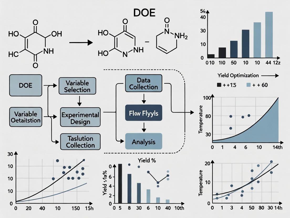
The DoE Optimization Workflow
The following diagram illustrates the logical, iterative process of optimizing a reaction using Design of Experiments.
Design of Experiments (DOE) is a systematic, statistical approach to process optimization that allows researchers to study the effects of multiple input factors on a desired output (response) simultaneously [9] [10]. In the context of improving low-yielding reactions in pharmaceutical research, DOE provides a structured methodology to efficiently identify key reaction parameters, optimize conditions, and understand complex factor interactions that traditional one-factor-at-a-time (OFAT) approaches often miss [9] [2].
For drug development professionals, implementing DOE enables more efficient screening of reaction conditions, reduces experimental time and costs, and provides a deeper understanding of the reaction landscape through statistical modeling [11]. This technical support center addresses common challenges researchers face when implementing DOE in their experimental workflows.
Core Principles and Terminology
Fundamental DOE Principles
DOE is built upon several key statistical principles that ensure experimental validity and reliability:
Randomization: The random assignment of experimental units to different treatment groups helps eliminate potential biases and distributes the effects of uncontrolled variables randomly across the experiment [12] [13]. For chemical reactions, this means performing experimental runs in a random order to mitigate the impact of environmental fluctuations or instrument drift.
Replication: Repeating experimental treatments allows researchers to estimate variability and improve the precision of effect estimates [12] [10]. In reaction optimization, replication helps distinguish significant factor effects from experimental noise.
Blocking: This technique accounts for known sources of nuisance variation by grouping experimental units into homogeneous blocks [12] [13]. For example, blocking by different reagent batches or laboratory technicians can remove these sources of variation from the experimental error.
Multifactorial Designs: Unlike OFAT approaches, DOE simultaneously varies multiple factors to efficiently explore the experimental space and detect interactions between factors [12] [2].
Key DOE Terminology
Table: Essential DOE Terminology for Reaction Optimization
| Term | Definition | Pharmaceutical Research Example |
|---|---|---|
| Factors | Input variables controlled by the researcher | Temperature, catalyst concentration, solvent type, reaction time |
| Levels | Specific values or settings assigned to a factor | Temperature: 25°C, 50°C, 75°C |
| Responses | Measurable outputs of experimental results | Reaction yield, purity, byproduct formation |
| Experimental Space | Multidimensional region defined by the ranges of all factors | All possible combinations of factor levels being studied |
| Interactions | Situation where the effect of one factor depends on the level of another factor | Temperature effect on yield varies with different solvent types |
| Confounding | When the effect of one factor cannot be distinguished from another | Unable to separate mixing speed effect from catalyst effect due to experimental design |
Experimental Design Types and Selection
Common DOE Designs
Different experimental designs serve specific purposes throughout the optimization process:
Screening Designs: Fractional factorial designs efficiently identify the most influential factors from a large set of potential variables with minimal experimental runs [14]. These are particularly valuable in early reaction development when many factors may affect the outcome.
Full Factorial Designs: These investigate all possible combinations of factors and their levels, allowing complete characterization of all main effects and interactions [10] [14]. While comprehensive, the number of runs grows exponentially with additional factors.
Response Surface Methodology (RSM): Designs such as Central Composite or Box-Behnken help model curvature in responses and locate optimal conditions [14]. These are ideal for final optimization stages when working with a few critical factors.
Space-Filling Designs: Useful when prior knowledge of the system is limited, these designs sample broadly across the experimental space without assumptions about the underlying model structure [14].
Design Selection Workflow
The following diagram illustrates the strategic selection of DOE designs throughout a typical reaction optimization campaign:
Troubleshooting Common DOE Implementation Issues
FAQ 1: How do I determine appropriate factor ranges for my reaction screening?
Problem: Researchers often struggle to define realistic minimum and maximum values for reaction factors, potentially missing optimal conditions or wasting resources on impractical regions.
Solution:
- Conduct preliminary scoping experiments to establish feasible ranges
- Utilize space-filling designs when prior knowledge is limited [14]
- Consider practical constraints (solvent boiling points, equipment limitations, safety concerns)
- For continuous factors (temperature, concentration), select ranges wide enough to detect effects but narrow enough to be practically relevant
Protocol: Start with a broad screening design using wide factor ranges, then progressively narrow the experimental space based on initial results. For a reaction with unknown optimal temperature, test from ambient to solvent reflux temperature rather than arbitrarily selecting a narrow window.
FAQ 2: My DOE results show unexpected factor interactions. How should I proceed?
Problem: Significant interaction effects between factors complicate interpretation and may contradict established mechanistic understanding of the reaction.
Solution:
- Verify the statistical significance of interactions through p-values and effect sizes
- Visualize interactions using interaction plots or 3D surface plots
- Consider whether interactions represent true chemical phenomena or confounding with uncontrolled variables
- If interactions are statistically significant and chemically plausible, incorporate them into your process model
Protocol: For a identified temperature-catalyst interaction, run confirmation experiments at the predicted optimal conditions and adjacent points to validate the response surface model [9].
FAQ 3: How can I effectively handle categorical factors like solvent or catalyst type in my DOE?
Problem: Traditional response surface methods assume continuous factors, creating challenges when including categorical variables like solvent choice or catalyst type.
Solution:
- Use specialized solvent maps based on principal component analysis (PCA) to incorporate solvent selection systematically [2]
- For catalyst screening, employ factorial designs that treat catalyst type as a categorical factor
- Consider split-plot designs when some factors are harder to change than others
Protocol: When optimizing solvent and temperature simultaneously, select solvents from different regions of solvent property space (polar, non-polar, protic, aprotic) rather than similar solvents to maximize information gain [2].
FAQ 4: What is the minimum number of experimental runs needed for reliable results?
Problem: Resource constraints often necessitate minimizing experimental runs while maintaining statistical validity.
Solution:
- For screening 5-8 factors, fractional factorial designs with 16-32 runs typically provide sufficient resolution [14]
- Include center points to detect curvature and estimate pure error
- Balance run numbers with required precision using power analysis
- Consider sequential experimentation rather than attempting complete optimization in one design
Protocol: When screening 6 factors for a new reaction, a resolution IV fractional factorial design with 16 runs plus 3 center points provides good ability to detect main effects and two-factor interactions while managing resource constraints.
FAQ 5: How do I address poor model fit or low predictive power in my DOE analysis?
Problem: The statistical model derived from experimental data shows poor fit statistics or fails validation experiments.
Solution:
- Check for outliers or influential points that may distort the model
- Verify that important factors weren't omitted from the original design
- Consider whether transformation of the response variable is appropriate
- Ensure the experimental region includes the optimum; otherwise, add experiments in promising directions
- Confirm measurement system reliability and response variability
Protocol: If R² value is low but significant factors are identified, add axial points to a factorial design to convert to a response surface design, providing additional information about curvature in the experimental region [14].
Factor-Response Relationships and Experimental Space
Mapping the Experimental Space
The experimental space represents all possible combinations of factor levels under investigation. Efficiently exploring this space requires understanding the relationship between factors and responses:
Quantitative Analysis of Factor Effects
Table: Calculating Main Effects and Interactions from a 2² Factorial Design
| Experiment | Temperature | Catalyst Loading | Yield (%) | Calculations |
|---|---|---|---|---|
| 1 | Low (-1) | Low (-1) | 65 | Main Effect Temp = (Y₂+Y₄)/2 - (Y₁+Y₃)/2 |
| 2 | High (+1) | Low (-1) | 78 | Main Effect Catalyst = (Y₃+Y₄)/2 - (Y₁+Y₂)/2 |
| 3 | Low (-1) | High (+1) | 72 | Interaction = (Y₁+Y₄)/2 - (Y₂+Y₃)/2 |
| 4 | High (+1) | High (+1) | 92 |
In this example, the main effect of temperature would be calculated as: (78+92)/2 - (65+72)/2 = 85 - 68.5 = 16.5%, indicating that increasing temperature generally improves yield. The interaction effect would be: (65+92)/2 - (78+72)/2 = 78.5 - 75 = 3.5%, suggesting a mild synergistic effect between temperature and catalyst loading [10].
Research Reagent Solutions for DOE Implementation
Table: Essential Materials and Tools for Reaction Optimization DOE
| Reagent/Equipment | Function in DOE | Application Example |
|---|---|---|
| Statistical Software | Experimental design generation and data analysis | JMP, Design-Expert, or R with specialized DOE packages |
| Automated Reactor Systems | Precise control of reaction parameters and high-throughput experimentation | Parallel reactor systems for simultaneous experimentation under different conditions |
| Solvent Libraries | Systematic variation of solvent environment | Curated solvent sets representing different polarity, hydrogen bonding, and polarizability parameters [2] |
| In Situ Analytics | Real-time reaction monitoring for multiple responses | FTIR, Raman spectroscopy, or HPLC for kinetic profiling |
| Design Templates | Standardized documentation of experimental plans | Customized spreadsheets or electronic lab notebooks with predefined DOE templates [10] |
Advanced DOE Applications in Pharmaceutical Research
Case Study: Reaction Optimization with Significant Interaction Effects
A pharmaceutical development team optimized a low-yielding SNAr reaction using DOE after traditional OFAT approaches failed to identify satisfactory conditions [2]. The team employed a fractional factorial design to screen six factors simultaneously:
- Factors included: solvent, temperature, base equivalence, nucleophile concentration, reaction time, and catalyst type
- Responses measured: yield, purity, and byproduct formation
- Key finding: Significant interaction between solvent and temperature explained why previous optimization attempts failed
- Outcome: Identified conditions that improved yield from 10% to 33% while reducing hazardous reagent use [11]
Sequential DOE for Multistep Optimization
For complex reactions with multiple competing responses (e.g., yield, purity, cost), a sequential approach is most effective:
- Screening Phase: Fractional factorial design to identify critical factors
- Optimization Phase: Response surface design around promising region
- Robustness Testing: Verify performance under small variations in factor settings
- Validation: Confirm optimal conditions with replication
This approach efficiently moves from broad screening to precise optimization while building comprehensive process understanding [14].
Implementing DOE principles for improving low-yielding reactions requires careful attention to factor selection, experimental design, and statistical analysis. By moving beyond one-factor-at-a-time approaches and embracing multifactorial experimentation with proper randomization, replication, and blocking, researchers can efficiently optimize complex reactions while developing deeper process understanding. The troubleshooting guidance provided in this technical support center addresses common implementation challenges, enabling more effective application of DOE methodologies in pharmaceutical research and development.
How DoE Efficiently Uncovers Hidden Factor Interactions
Why didn't my One-Factor-at-a-Time (OFAT) experiment find the optimal reaction conditions?
OFAT experiments, where you change only one variable while holding others constant, are inefficient and cannot detect interactions between factors [9] [15]. An interaction occurs when the effect of one factor (e.g., Temperature) on the response (e.g., Yield) depends on the level of another factor (e.g., pH) [9].
For example, an OFAT approach to maximize a chemical yield might conclude that a Temperature of 30°C and a pH of 6 is optimal, achieving an 86% yield [9]. However, a properly designed Design of Experiments (DOE) that systematically varies both factors together found the true optimum was at 45°C and a pH of 7, with a predicted yield of 92% [9]. The OFAT method completely missed this because it could not see how Temperature and pH interact [9].
What is a Design of Experiments (DOE) and how does it find interactions?
DOE is a systematic, statistical approach for planning, conducting, and analyzing controlled tests to evaluate the factors that influence a process [15]. Unlike OFAT, a DOE changes multiple factors simultaneously according to a structured plan (a design matrix) [15]. This allows you to:
- Estimate the individual effect of each factor on your response.
- Identify and quantify interactions between factors.
- Develop a predictive model to find optimal factor settings, even between the tested points [9].
The following diagram illustrates the core workflow of a DOE, from design to discovery.
How do I set up a basic DOE to test for interactions?
For a two-factor system, a full factorial design is an excellent starting point. It tests all possible combinations of the factors' levels [15].
Step-by-Step Protocol: Two-Factor Full Factorial DOE
- Define Factors and Levels: Select two factors you want to investigate (e.g., Reaction Temperature and Catalyst Concentration). Choose a realistic "low" and "high" level for each factor to investigate [15].
- Create the Design Matrix: This matrix outlines the exact experimental runs needed. For two factors at two levels, you need 2² = 4 runs [15].
- Run Experiments: Perform the experiments in a randomized order to avoid confounding the results with unknown, time-related variables [15].
- Analyze the Results: Calculate the main effects and the interaction effect from your experimental data.
The table below shows a sample design matrix and results for a chemical reaction, where the response is Yield (%).
Table 1: Design Matrix and Results for a Two-Factor DOE
| Experimental Run | Temperature (°C) | Catalyst Concentration (%) | Yield (%) |
|---|---|---|---|
| 1 | 100 (Low) | 1.0 (Low) | 21 |
| 2 | 100 (Low) | 2.0 (High) | 42 |
| 3 | 200 (High) | 1.0 (Low) | 51 |
| 4 | 200 (High) | 2.0 (High) | 57 |
Using the data in Table 1, you can calculate the effects [15]:
- Main Effect of Temperature: (Average Yield at High Temp) - (Average Yield at Low Temp) = [(51 + 57)/2] - [(21 + 42)/2] = 54 - 31.5 = +22.5%
- Main Effect of Concentration: (Average Yield at High Conc.) - (Average Yield at Low Conc.) = [(42 + 57)/2] - [(21 + 51)/2] = 49.5 - 36 = +13.5%
To calculate the interaction effect, you need to expand the design matrix to include an interaction column. The coded levels for the interaction are found by multiplying the levels of Temperature and Concentration for each run [15].
Table 2: Design Matrix with Interaction Term
| Run | Temp (T) | Conc (C) | T x C Interaction | Yield (%) |
|---|---|---|---|---|
| 1 | -1 (Low) | -1 (Low) | (-1) * (-1) = +1 | 21 |
| 2 | -1 (Low) | +1 (High) | (-1) * (+1) = -1 | 42 |
| 3 | +1 (High) | -1 (Low) | (+1) * (-1) = -1 | 51 |
| 4 | +1 (High) | +1 (High) | (+1) * (+1) = +1 | 57 |
- Interaction Effect (T x C): (Average Yield where Interaction is +1) - (Average Yield where Interaction is -1) = [(21 + 57)/2] - [(42 + 51)/2] = 39 - 46.5 = -7.5%
This negative interaction effect reveals that the effect of temperature is less pronounced at higher catalyst concentrations, and vice versa. This hidden relationship is impossible to detect with OFAT. The diagram below visualizes this concept.
What are the practical steps for executing a successful DOE?
Follow this five-step protocol to ensure your DOE is robust and provides actionable results [6].
- Identify and Isolate Variables: Test one variable or solution at a time to pinpoint the most effective change. Avoid making multiple modifications simultaneously, as this complicates analysis and can introduce new issues [6].
- Determine Sample Size: Test enough units for statistical significance. As a rule of thumb, to validate a fix for an issue with a failure rate of p, you should test at least n = 3/p units with zero failures to be 95% confident (⍺=0.05) the problem is solved. For a 10% failure rate, plan to test 30 units [6].
- Execute with Vigilance: Keep extremely accurate records and be hyper-vigilant during assembly to prevent kitting and configuration errors that can invalidate your results [6].
- Validate in the Real World: Ensure your test setup accurately simulates real-world conditions. A test is only valuable if its results predict actual performance in the field [6].
- Deploy and Confirm at Scale: After finding a solution, validate the change at full scale with all relevant performance and reliability tests before final implementation [6].
The Scientist's Toolkit: Essential DOE Research Reagents
Table 3: Key Components for a Successful DOE Initiative
| Item | Function in DOE |
|---|---|
| Design Matrix | A structured table that defines the set of experimental runs. It is the blueprint for your DOE, ensuring efficient and systematic data collection [15]. |
| Statistical Software | Tools (e.g., JMP, R, Python libraries) used to randomize the run order, analyze the results, calculate effects, build predictive models, and visualize interaction effects [9]. |
| Randomization Protocol | A procedure to run experimental trials in a random sequence. This is critical to eliminate the influence of confounding, uncontrolled variables (e.g., ambient humidity, reagent age) [15]. |
| Predictive Model | A mathematical equation (often a polynomial) that describes the relationship between your factors and the response. It allows you to predict outcomes and find optima within the experimental region [9]. |
| Response Surface Plot | A 3D visualization of the predictive model. This graph makes it easy to see the shape of the response and identify interactions and optimal settings [9]. |
Frequently Asked Questions (FAQs)
What is the primary advantage of using DoE over a traditional One-Variable-at-a-Time (OVAT) approach for optimizing a low-yielding reaction?
The primary advantage is the ability to efficiently identify optimal conditions and understand interactions between multiple factors simultaneously. A traditional OVAT approach, where only one variable is changed while others are held constant, can be inefficient and may miss the true optimum due to factor interactions [2]. In contrast, DoE is a systematic approach that allows scientists to screen a large number of reaction parameters in a relatively small number of experiments, enabling them to model the effect of each variable and their interactions to find the best possible outcome [11] [2].
A DoE study suggested that higher temperature and lower reagent equivalents are optimal for my reaction, which contradicts my initial hypothesis. Should I trust the model?
Yes, you should initially trust the model, as this is a common and powerful outcome of a DoE analysis. DoE is designed to uncover these non-intuitive interactions that are easily missed with OVAT. The statistical model is based on empirical data from your experiments [2]. The next step should be to run a verification experiment at the predicted optimal conditions (high temperature, low reagent equivalents) to confirm the model's accuracy. A successful verification experiment, which yields the predicted result, validates the model and provides a robust set of conditions [2].
My chemical reaction generates multiple problematic byproducts. Can DoE help with this beyond just improving yield?
Absolutely. DoE is exceptionally well-suited for improving reaction selectivity and reducing byproducts. By systematically varying parameters and analyzing the outcomes, you can identify conditions that favor the formation of your desired product while suppressing the pathways that lead to byproducts [11]. For example, one case study involved a reaction generating five structurally similar byproducts. A DoE exercise was used to adjust reaction conditions, which not only increased the desired product yield three-fold (from 10% to 33%) but also reduced the proportion of these hard-to-remove byproducts [11].
How can I use DoE to find a safer or more sustainable solvent for my reaction?
DoE can be coupled with a "solvent map" to systematically explore solvent space. Instead of testing a random selection of solvents, a solvent map based on Principal Component Analysis (PCA) groups solvents by their key physical properties [2]. You can select a few solvents from different regions of this map for your DoE screening. The results will show you which area of solvent space (e.g., polar aprotic, non-polar, etc.) is optimal for your reaction, allowing you to identify high-performing, safer, or more sustainable solvents you might not have otherwise considered [2].
After implementing new conditions from a DoE, how can I ensure my process remains robust and consistent over time?
Once optimal conditions are identified, Statistical Process Control (SPC) is the ideal methodology for ensuring long-term process robustness and consistency [16]. SPC uses control charts to monitor process behavior over time, distinguishing between common cause variation (inherent to the process) and special cause variation (indicating a problem) [16]. This data-driven approach allows for proactive problem-solving, helping you maintain control over your optimized process and prevent deviations before they lead to failed batches or variations in product quality [16] [17].
Troubleshooting Guide
Poor Model Fit or Insignificant Factors
Symptoms: The statistical model from your DoE has a low R² value (poor predictive power), or analysis of variance (ANOVA) shows that most factors are not statistically significant.
| Potential Cause | Solution |
|---|---|
| Insufficient factor range | The chosen high and low values for your factors were too close together, resulting in a signal that is too weak to detect over the background noise. Widen the ranges for key factors in a subsequent DoE round. |
| High experimental noise | Uncontrolled variables or measurement errors are obscuring the effects of your factors. Improve experimental consistency, ensure proper calibration of equipment, and consider replicating center points to better estimate noise. |
| Missing key factors | The variables you chose to study may not be the most impactful ones for this specific reaction. Conduct further fundamental research on the reaction mechanism to identify more critical factors to test. |
Failure to Verify the Model's Predictions
Symptoms: When you run a new experiment at the optimal conditions predicted by the DoE model, the result (e.g., yield) does not match the model's prediction.
| Potential Cause | Solution |
|---|---|
| Model interpolation | The verification point might lie far outside the experimental region used to build the model. Models are reliable for interpolation (within the factor space studied) but not for extrapolation. Ensure your verification point is within the bounds of your original experimental design. |
| Presence of curvature | The model may be too simple (e.g., linear) for a process that has significant curvature. Add center points to your initial design to detect curvature. If present, augment your design with additional experiments to create a higher-order (e.g., quadratic) model. |
| Uncontrolled factor drift | An unmeasured variable (e.g., raw material purity, ambient humidity) changed between the initial DoE and the verification run. Strictly control laboratory conditions and document all potential sources of variation. |
High Variation in Replicate Experiments
Symptoms: Replicate runs of the same experimental conditions (e.g., center points) show unacceptably high variability.
| Potential Cause | Solution |
|---|---|
| Inconsistent procedure | The experimental protocol may allow for too much interpreter judgment. Create a highly detailed, step-by-step procedure and ensure all lab personnel are trained on it. |
| Unreliable analytical method | The method used to measure the output (e.g., yield, purity) may not be precise. Perform a method validation to ensure the analytical technique is fit for purpose before starting the DoE. |
| Poor raw material control | The starting materials or reagents may have inconsistent quality or purity. Source materials from a single, reliable batch for the entire DoE study to eliminate this source of variation. |
Quantitative Benefits of DoE
The table below summarizes documented quantitative benefits of implementing DoE for process optimization.
| Benefit | Metric | Quantitative Improvement | Context / Source |
|---|---|---|---|
| Yield Improvement | Percentage Yield | Increased from 10% to 33% (3-fold increase) | Optimization of a complex API step with multiple byproducts [11]. |
| Resource Efficiency | Raw Material Usage | Reduced quantity of required materials | DoE-optimized conditions minimized use of expensive/hazardous reagents [11]. |
| Process Efficiency | Hazardous Chemical Use | Reduced use of hazardous chemicals | Mitigated risks by identifying safer process windows [11]. |
| Experimental Efficiency | Number of Experiments to Optimize | 19 experiments to explore up to 8 factors with interactions | Resolution IV DoE design versus dozens to hundreds of OVAT experiments [2]. |
Experimental Protocol: A Basic DoE Workflow for Reaction Optimization
Objective: To systematically optimize a low-yielding chemical reaction by evaluating the impact of and interactions between three critical factors: Reaction Temperature, Catalyst Loading, and Solvent Type.
Step 1: Define the Problem and Objectives
- Clearly state the primary response (e.g., reaction yield).
- Define secondary responses (e.g., purity, byproduct level).
Step 2: Select Factors and Ranges
- Factor 1: Temperature. Range: 50°C to 100°C.
- Factor 2: Catalyst Loading. Range: 1 mol% to 5 mol%.
- Factor 3: Solvent. Choose 3-4 solvents from different regions of a solvent property map (e.g., Toluene, THF, DMF) [2].
Step 3: Select an Experimental Design
- A full factorial design is recommended for 3 factors. This requires 8 experiments (2³) plus 2-3 replicates of the center point to estimate experimental error.
Step 4: Run the Experiments
- Execute all experiments in a randomized order to avoid systematic bias.
- Adhere to a strict, written procedure for consistency.
Step 5: Analyze the Data
- Use statistical software to perform ANOVA.
- Identify which factors and interactions are significant.
- Generate a statistical model and contour plots to visualize the relationship between factors and the response.
Step 6: Validate the Model
- Run 1-2 additional experiments at the predicted optimal conditions.
- Compare the actual result with the model's prediction. A close match confirms a reliable model.
Process Optimization Workflow
Research Reagent Solutions
The following table details key materials and their functions in a typical DoE study for reaction optimization.
| Item | Function in DoE Context |
|---|---|
| Solvent Map | A statistical tool (based on Principal Component Analysis) that groups solvents by physical properties, enabling systematic selection of a diverse set of solvents to screen in a DoE, moving beyond trial and error [2]. |
| Catalyst Library | A collection of commercially available or synthetically accessible catalysts. A DoE can efficiently screen different metal centers or ligand structures to identify the most active and selective catalyst for a transformation. |
| Statistical Software | Essential for generating the set of experiments for a given design (e.g., factorial, response surface) and for analyzing the resulting data to build predictive models and identify significant factors and interactions [11]. |
| Design Matrix | The pre-defined set of experimental conditions generated by statistical software. It serves as the rigorous protocol for the DoE study, ensuring efficient and systematic data collection [11] [2]. |
Defining the Problem and Setting Clear, Measurable Objectives for Yield Improvement
Frequently Asked Questions: Problem Definition and Objectives
Q1: Why is it crucial to define the problem and set objectives before starting a Design of Experiments (DoE) for a low-yielding reaction?
A clearly defined problem and objective are the foundation of a successful DoE. Without them, experiments can become unfocused, waste resources, and fail to identify a solution. A precise objective ensures that the experimental design is structured to collect the right data to solve your specific yield problem [18] [19]. It guides the selection of factors to study and the responses to measure, keeping the project aligned with the ultimate goal of yield improvement.
Q2: How can I determine if my low-yielding reaction is a good candidate for a DoE study?
A reaction is a good candidate for DoE if it is stable and repeatable, even if the yield is low. Before starting DoE, you should ensure that the process is under statistical control. This means that when you run the reaction multiple times at the same conditions, the results are consistent. If the yield varies wildly under identical conditions, the underlying process instability must be addressed first, as it will be difficult to distinguish the effect of your experimental factors from random process noise [18].
Q3: What are some common mistakes when setting objectives for yield improvement?
Common mistakes include:
- Vague Goals: Setting an objective like "improve yield" is not measurable. A good objective is specific, such as "increase the reaction yield from 20% to at least 40%."
- Ignoring Process Stability: Conducting a DoE on an unstable process, leading to unreliable results [18].
- Ignoring Critical Responses: Focusing only on yield while ignoring other critical responses like purity, byproduct formation, or cost. A yield increase is not beneficial if it leads to an impure product that is difficult to isolate [11] [19].
Q4: What does a well-structured, measurable objective for a yield improvement DoE look like?
A well-structured objective is Specific, Measurable, Achievable, Relevant, and Time-bound (SMART). For example: "To identify and model the effect of temperature, catalyst charge, and reaction time on the yield and purity of API XYZ-123. The goal is to define a design space that provides a consistent yield of >85% with a purity of >99.5% and reduces the current level of critical byproduct ABC by 90%, within the next 4 weeks." This objective clearly states the factors, responses, and desired targets [11] [19].
Troubleshooting Guide: Problem Definition & Objective Setting
This guide helps you diagnose and resolve common issues encountered during the initial phase of a yield improvement project.
| Problem Area | Symptom | Likely Cause | Corrective Action |
|---|---|---|---|
| Unclear Problem Scope | The team cannot agree on the primary goal; the experiment seems to be expanding to cover too many things. | The problem has not been sufficiently bounded or broken down. | Refocus on the primary issue. Use tools like a SIPOC diagram (Suppliers, Inputs, Process, Outputs, Customers) to map the process and isolate the step with the yield problem [3]. |
| Unmeasurable Objective | Success cannot be quantified. There is debate after the experiment about whether the goal was met. | The objective lacks specific, numerical targets for key responses. | Define measurable responses. Instead of "improve yield," set a target like "achieve a mean yield of 35%." Also, define measurable targets for other Critical Quality Attributes (e.g., reduce specified byproduct to <1.5%) [19]. |
| Unstable Baseline | High variation in yield even when reaction parameters are kept constant. | The process is influenced by uncontrolled lurking variables (e.g., raw material variability, equipment calibration drift, operator technique) [3] [18]. | Stabilize the process first. Use Statistical Process Control (SPC) charts to establish a baseline. Control and standardize all input materials, equipment settings, and operator procedures before beginning the DoE [18]. |
| Overlooked Interactions | The optimized conditions from the DoE do not perform as expected in validation runs. | The experimental objective was too narrow, focusing only on main effects and ignoring how factors interact (e.g., the effect of temperature might depend on the catalyst charge) [11]. | Include interaction effects in the objective. State that the goal is to understand not just the main effects of factors but also their two-factor interactions on the yield [11] [20]. |
Experimental Protocol: Establishing a Baseline for Yield Improvement
Before designing any experiments, you must establish a reliable baseline for your low-yielding reaction.
Objective: To confirm process stability and determine the baseline mean and variability of the reaction yield under current standard operating conditions.
Methodology:
- Standardize Conditions: Document and fix all reaction parameters (e.g., reagent concentrations, stirring speed, temperature, reaction vessel) based on existing procedures [18].
- Replicate Runs: Perform a minimum of n=5 independent experimental runs using the exact standardized conditions. A larger sample size (e.g., n=10) will provide a more reliable estimate of variability.
- Randomize Order: Execute the runs in a random order to protect against unknown lurking variables that may change over time [3] [21].
- Execute and Measure: Carry out each run carefully, ensuring the product is isolated and purified using the standard workup procedure. Measure the final yield for each run.
Data Analysis:
- Calculate the mean yield and standard deviation.
- Create a control chart (e.g., an Individuals and Moving Range chart) with the yield data to assess statistical process control. A process is considered stable if no points fall outside the control limits and no non-random patterns are observed [3] [18].
Example of Baseline Data Table:
| Run Order | Yield (%) | Notes |
|---|---|---|
| 1 | 22.5 | |
| 2 | 24.1 | |
| 3 | 19.8 | Material from new batch used |
| 4 | 23.3 | |
| 5 | 20.5 | |
| Mean | 22.0 | |
| Std. Dev. | 1.8 |
In this example, the low yield of Run 3 could be investigated as a potential special cause related to the new material batch, highlighting the importance of controlling inputs [18].
The Scientist's Toolkit: Key Research Reagent Solutions
Selecting and controlling reagents is critical for a successful yield improvement study. The table below lists essential material categories and their functions.
| Research Reagent / Material | Function in Optimization | Key Consideration for DoE |
|---|---|---|
| High-Purity Starting Materials | The foundation of the reaction; impurities can catalyze side reactions, consuming reactants and lowering yield. | Use a single, consistent batch for the entire DoE to eliminate raw material variability as a source of noise [18]. |
| Catalysts | Substances that increase the reaction rate and selectivity without being consumed, directly impacting yield and byproduct formation. | A primary factor to study. Systematically vary the type (if screening) or charge (mol%) as a factor in the experimental design [11]. |
| Solvents | The medium in which the reaction occurs; can influence reaction rate, mechanism, and selectivity. | A key factor to study. Vary solvent identity (e.g., polarity, protic/aprotic) or volume to find optimal reaction conditions. |
| Reagents & Ligands | Substances used in stoichiometric amounts or to modify catalyst properties, critical for achieving high selectivity. | Systematically test different reagents or ligand structures to suppress byproduct pathways and improve yield [11]. |
DoE Objective Setting Workflow
The following diagram outlines the logical workflow for moving from a vague problem to a clear, actionable DoE objective.
Your Practical Playbook: Implementing Screening and Optimization DoE Designs
FAQs and Troubleshooting Guide
FAQ 1: When should I use a Full Factorial design over a Fractional Factorial design for my reaction optimization?
| Design Type | When to Use | Key Advantages | Key Limitations |
|---|---|---|---|
| Full Factorial | - Number of factors (k) is small (e.g., ≤ 4) [3] [22]- A complete understanding of all interaction effects is required [22]- Sufficient resources (time, materials) are available for a large number of runs | - Provides comprehensive insights into all main effects and interactions [22]- Unambiguously reveals complex, non-linear relationships between variables [22] | - Number of runs grows exponentially with factors (2^k for 2-level designs) [22]- Can be resource-intensive (cost, time, materials) [22] |
| Fractional Factorial | - Screening a larger number of factors (e.g., 5 or more) to identify the most influential ones [3] [23]- Resources are limited, and experimental efficiency is critical [24] [23] | - Drastically reduces the number of runs required (e.g., a half or quarter fraction) [23]- Highly efficient for identifying vital few significant factors [23] | - Introduces aliasing (some effects are confounded and cannot be separated) [23]- Lower resolution designs may confound main effects with two-factor interactions [23] |
Troubleshooting: A common mistake is using a Resolution III fractional factorial design, where main effects are confounded with two-factor interactions, making interpretation difficult. If your initial fractional factorial results are ambiguous, consider folding the design—a technique that adds a mirror-image set of runs to break the alias chains and separate these confounded effects [23].
FAQ 2: What is a Definitive Screening Design (DSD) and when is it most beneficial?
Answer: A Definitive Screening Design (DSD) is an advanced, highly efficient experimental design that allows you to screen a large number of factors while requiring a very small number of runs. Its key differentiator is the ability to identify active factors and estimate their curvilinear (quadratic) effects simultaneously, which is not possible with standard two-level screening designs [3].
When to use a DSD:
- You need to screen many factors (e.g., 6 or more) [3].
- You suspect the relationship between a factor and your response (like reaction yield) might be non-linear [3].
- Experimental runs are exceptionally expensive or time-consuming, and you need the maximum information from a minimal number of experiments [3].
Troubleshooting: A significant advantage of DSDs is that their analysis is often more straightforward than that of highly fractionated factorial designs, as main effects are not confounded with each other or with two-factor interactions [3]. This makes them an excellent choice for researchers who may be less familiar with complex alias structures.
FAQ 3: My initial DoE yielded ambiguous results. How can I augment my design to get clearer answers?
Answer: If your initial design, particularly a fractional factorial, has confounded effects that you cannot separate, you do not need to abandon your work. You can augment your design with additional runs [23].
- Folding a Fractional Factorial Design: This involves adding a new set of runs that is a mirror image (where factor levels are swapped) of your original design. Folding on all factors can separate all main effects from two-factor interactions in a Resolution III design [23].
- Sequential Experimentation: DoE is often most effective when done sequentially. Start with a screening design (e.g., Fractional Factorial or DSD) to identify vital factors. Then, use a more focused design, like a Response Surface Methodology (RSM), to model curvature and find the precise optimum around those vital factors [24].
Experimental Protocol: A Sequential DoE Strategy for Reaction Optimization
This protocol outlines a two-stage approach to efficiently optimize a low-yielding chemical reaction, moving from screening to optimization.
Stage 1: Factor Screening with a Definitive Screening Design (DSD)
- Define Factors and Ranges: List all potential factors (e.g., temperature, catalyst loading, solvent, concentration) and define a high and low level for each that represents a reasonable but wide operating range [25].
- Generate the Design: Use statistical software (e.g., JMP, Minitab, R with the
daewrpackage) to create a DSD for your number of factors [3]. - Execute Experiments: Run the experiments in a fully randomized order to mitigate the effects of lurking variables [22] [26].
- Analyze Data: Fit a model to identify which factors have a statistically significant main or quadratic effect on your response (e.g., reaction yield).
Stage 2: Response Optimization with a Full Factorial or RSM Design
- Select Vital Factors: Choose the 2 or 3 most significant factors identified in Stage 1.
- Create Optimization Design:
- Execute and Analyze: Run the experiments in random order. Use regression analysis and ANOVA to build a predictive model and identify the optimal factor settings that maximize yield [22].
The Scientist's Toolkit: Essential Research Reagent Solutions
| Item | Function in DoE for Reaction Optimization |
|---|---|
| Statistical Software (e.g., JMP, Minitab, R) | Used to generate the experimental design matrix, randomize the run order, and perform statistical analysis (ANOVA, regression) to interpret results [24]. |
| Solvent Map (via Principal Component Analysis) | A plot that groups solvents by their physical properties. Allows for the systematic selection of a few, diverse solvents to efficiently represent the entire "solvent space" in a DoE, moving beyond trial-and-error [2]. |
| Center Points | Replicate experiments run at the midpoint level of all continuous factors. They are essential for estimating pure experimental error and testing for the presence of curvature in the response surface [27] [2]. |
| "Folded" Design | A follow-up set of experimental runs that is a mirror image of an initial fractional factorial design. Used to resolve ambiguity by separating confounded effects (aliases) [23]. |
Workflow Diagram: Selecting Your Experimental Design
The diagram below outlines a logical decision pathway to help you select the most appropriate experimental design for your project.
Troubleshooting Guides
Why is my screening design not identifying any significant factors?
This often occurs due to incorrect factor ranges or a missing critical factor.
Potential Cause & Solution: The chosen ranges for your factors might be too narrow to produce a detectable effect on the response. Re-visit your process knowledge and consider widening the high and low levels for your factors. Additionally, use a cause-and-effect diagram in your planning phase to ensure no critical factor has been overlooked [3].
Verification Protocol:
- Check the model's analysis of variance (ANOVA). A low model F-value and a high p-value indicate the model is not significant.
- Examine the Pareto chart of effects; no factors will exceed the significance line.
- If resources allow, re-run the screening design with wider factor ranges.
How do I handle a large number of potential factors with a limited experimental budget?
Use highly fractional designs like Plackett-Burman or Definitive Screening Designs (DSD).
Potential Cause & Solution: A full factorial design for many factors is prohibitively large. A Plackett-Burman design is an efficient screening design that assumes interactions are negligible compared to main effects, allowing you to screen a large number of factors (N-1 factors in N runs, where N is a multiple of 4) [19] [28]. For more advanced analysis, Definitive Screening Designs can handle a large number of factors with three levels each in a minimal number of runs and allow for the detection of curvature [3].
Verification Protocol:
- Select a design type (e.g., Plackett-Burman) in your statistical software (e.g., JMP, Minitab).
- Specify all your potential factors and set them to two levels.
- The software will generate an experimental run sheet with a fraction of the runs required for a full factorial study. Execute these runs [28].
What does significant "lack of fit" mean in my screening design analysis?
This indicates your linear model might be missing important curvature, often from a quadratic effect.
Potential Cause & Solution: The relationship between a factor and your response is not linear but curved. This can be detected by including center points in your two-level screening design. A significant lack of fit test suggests you may need to move to an optimization design, like a Response Surface Methodology (RSM), that can model this curvature [28].
Verification Protocol:
- Ensure your screening design included 3-5 replicate runs at the center point (all continuous factors set to their mid-level).
- In your software, run the analysis and check the "Lack of Fit" p-value in the ANOVA output. A p-value less than 0.05 indicates significant lack of fit.
- The design can be augmented with axial points to create a central composite design for response surface analysis.
My screening results are inconsistent with known process knowledge. What went wrong?
This can stem from assembly errors, uncontrolled noise variables, or a flawed testing method.
Potential Cause & Solution: Errors during the assembly of experimental units can introduce unexpected variation. Be hyper-vigilant during assembly to ensure each unit is built to the exact specification for its run [6]. Furthermore, an uncontrolled lurking variable (e.g., raw material batch, ambient humidity) may be influencing your results. Finally, validate that your test method accurately simulates real-world conditions [6].
Verification Protocol:
- Review assembly records and procedures for kitting errors.
- Brainstorm potential lurking variables using a SIPOC (Suppliers, Inputs, Process, Outputs, Customers) diagram and control them in future experiments [3].
- Correlate your test results with a known, real-world outcome to validate your test method.
Frequently Asked Questions (FAQs)
Q1: When should I use a screening design versus an optimization design? Screening designs are used early in experimentation when you have many potential factors and need to identify the "vital few" that have the largest impact. Optimization designs (e.g., RSM) are used later to model the response in detail and find the precise factor settings that produce an optimal result after the important factors are known [28] [3].
Q2: How many experimental runs do I need for a screening design? The number of runs depends on the number of factors and the specific design. For example, a Plackett-Burman design can screen up to 11 factors in 12 runs, or 7 factors in 8 runs. Definitive Screening Designs can screen k factors in 2k+1 runs [3]. The key is that it is a fraction of the full factorial, which would require 2^k runs.
Q3: Can screening designs detect interactions between factors? Some can, but with limitations. Traditional screening designs like Plackett-Burman assume interactions are negligible. However, modern designs like Definitive Screening Designs (DSD) or certain fractional factorials have better capabilities to identify active two-factor interactions without being confounded with main effects, which is a significant advantage [28] [3].
Q4: What is the "sparsity of effects" principle? This is a key principle underlying screening designs. It states that in most systems, only a relatively small number of factors (the "vital few") will have significant main effects, while most will have little to no effect (the "trivial many") [28]. Screening designs are built to efficiently find these vital few.
Q5: Our one-variable-at-a-time (OVAT) approach has worked so far. Why switch to screening designs? OVAT is inefficient and can miss critical interactions between factors. For example, changing the level of Factor A might have a different effect depending on the setting of Factor B. A screening design varies all factors simultaneously in a controlled pattern, allowing you to detect these interactions and find better optima with fewer total experiments [29]. A study on copper-mediated fluorination showed that DoE provided a more than two-fold increase in experimental efficiency compared to the OVAT approach [29].
Experimental Protocols
Protocol 1: Setting Up a Definitive Screening Design (DSD) for a Chemical Reaction
This protocol outlines the steps for using a DSD to screen factors affecting the yield of a low-yielding organic synthesis reaction.
1. Objective Definition:
- Primary Goal: Identify factors significantly affecting the reaction yield (%).
- Secondary Goal: Check for any strong two-factor interactions and curvature.
2. Factor and Level Selection:
- Select 5 continuous factors believed to influence the reaction (e.g., Temperature, Catalyst Amount, Reaction Time, Solvent Volume, Stirring Rate).
- Set each factor to three levels: Low (-1), Middle (0), and High (+1). The middle level is critical for detecting curvature.
3. Experimental Design Generation:
- Using statistical software (e.g., JMP Pro), select the "Definitive Screening Design" type.
- Input the 5 factors. The software will automatically generate a design with 2*5 + 1 = 11 experimental runs.
- Randomize the run order to minimize the impact of lurking variables.
4. Execution and Data Collection:
- Conduct each of the 11 reactions according to the randomized run sheet.
- Precisely control and record all factor levels for each run.
- Measure and record the response (reaction yield) for each run using a consistent analytical method (e.g., HPLC).
5. Data Analysis:
- Input the response data into the software.
- Fit a model using the software's automated analysis for DSDs.
- Identify significant factors by examining the Pareto chart and the p-values in the ANOVA table (typically p < 0.05).
- Use the model to understand the direction of each factor's effect and to predict settings for follow-up optimization.
Protocol 2: Executing a Plackett-Burman Screening Design for a Formulation
This protocol is for a formulation scientist needing to screen many excipients and process parameters to improve drug dissolution.
1. Objective Definition:
- Goal: Screen 7 formulation factors to identify those critically affecting the dissolution similarity factor (f2).
2. Factor and Level Selection:
- Choose 7 factors (e.g., Polymer Type [A or B], Binder Level [Low/High], Disintegrant Level [Low/High], Compression Force [Low/High], Lubricant Amount [Low/High], Mixing Time [Low/High], Moisture Content [Low/High]).
- Set each to two levels.
3. Experimental Design Generation:
- In software like Minitab or MODDE, select a Plackett-Burman design for 7 factors.
- The design will likely require 8 experimental runs.
- Include 2 additional center point runs (for continuous factors) to check for curvature and estimate pure error, for a total of 10 runs.
- Randomize the run order.
4. Execution and Data Collection:
- Prepare 10 batches of the formulation according to the design matrix.
- Perform dissolution testing on all batches according to pharmacopeial standards, collecting data at multiple time points.
- Calculate the f2 value for each batch against a reference profile.
5. Data Analysis:
- Perform multiple linear regression to fit a main-effects-only model with the f2 value as the response.
- The half-normal plot or a Pareto chart of effects will visually highlight the most influential factors.
- Factors far from the "noise" line or with low p-values (<0.05) are considered significant and should be investigated further in an optimization study.
Data Presentation
Table 1: Comparison of Common Screening Design Types
| Design Type | Number of Runs for k Factors | Can Estimate Main Effects? | Can Estimate Interactions? | Can Detect Curvature? | Best Use Case |
|---|---|---|---|---|---|
| Plackett-Burman | N (multiple of 4), e.g., 8 runs for 7 factors | Yes | No (assumed negligible) | No (requires center points) | Initial screening of a very large number of factors with a tight budget [19] [28] |
| Fractional Factorial (2^(k-p)) | 2^(k-p) (e.g., 8 runs for 4 factors) | Yes | Yes, but some are confounded (aliased) with other effects | No (requires center points) | Screening when some information on two-factor interactions is needed [3] |
| Definitive Screening Design (DSD) | 2k + 1 | Yes | Yes, all two-factor interactions are clear of main effects | Yes | The modern recommended choice for screening 6-12 factors; highly efficient and informative [3] |
Table 2: Research Reagent Solutions for a Model Copper-Mediated Radiofluorination
This table details key materials used in a model reaction optimized via a screening design, as referenced in the literature [29].
| Reagent / Material | Function in the Experiment |
|---|---|
| Arylstannane Precursor | The substrate molecule that undergoes radiofluorination; its structure is a key variable [29]. |
| Copper Mediator (e.g., Cu(OTf)₂(py)₄) | Facilitates the transfer of the fluoride ion to the aromatic ring, essential for the reaction to proceed [29]. |
| [[¹⁸F]Fluoride Ion | The radioactive isotope introduced into the precursor molecule to create the PET tracer [29]. |
| Anion Exchange Cartridge (QMA) | Used to process and purify the cyclotron-produced [[¹⁸F]fluoride ion before the reaction [29]. |
| Base (e.g., K₂CO₃) | Used to elute the [[¹⁸F]fluoride from the QMA cartridge and make it chemically reactive [29]. |
| Azeotropic Solvent (e.g., MeCN) | Used to dry the [[¹⁸F]fluoride to remove water, which is critical for achieving high reactivity [29]. |
| Organic Solvent (e.g., DMF, DMSO) | The reaction medium that dissolves all components and provides a suitable environment for the fluorination [29]. |
Visualizations
Screening Design Selection Workflow
Screening Design Conceptual Framework
Advanced Optimization with Response Surface Methodology (RSM) and Central Composite Designs
Response Surface Methodology (RSM) is a collection of statistical techniques for designing experiments, building models, and exploring factor relationships to optimize processes. Within RSM, Central Composite Design (CCD) is a widely used experimental design for fitting second-order models, which are essential for identifying optimal conditions in complex chemical processes. For researchers working on improving low-yielding reactions, this sequential methodology provides a structured path from initial screening to final optimization, moving efficiently through experimental space to find factor combinations that maximize desired outcomes. This technical guide addresses common implementation challenges and provides frameworks for successful application in pharmaceutical development contexts.
RSM Fundamentals: Core Concepts FAQ
What is the fundamental objective of Response Surface Methodology? RSM aims to find the optimal factor level combinations that achieve a specific process goal, such as maximum yield, minimum cost, or target specifications. Unlike screening designs that identify important factors, RSM focuses on optimization, often involving second-order models to capture curvature in the response surface and locate stationary points [30].
How does RSM improve upon the "one variable at a time" (OVAT) approach? Traditional OVAT optimization varies one factor while holding others constant, which frequently fails to identify true optimum conditions when factor interactions exist. RSM varies multiple factors simultaneously, efficiently exploring "reaction space" and capturing interaction effects that OVAT approaches miss [2]. For example, temperature and reagent equivalents might interact such that higher temperatures allow fewer equivalents to achieve better yields—a relationship OVAT would likely overlook.
What is the typical sequential process for implementing RSM? RSM generally follows a staged approach:
- Screening: Identify significant factors using first-order designs
- Steepest Ascent/Descent: March toward the optimum region using linear models
- Optimization: Characterize the optimum region with second-order models when curvature becomes significant [30]
This progression from initial first-order model ((y = \beta0 + \beta1x1 + \beta2x2 + \varepsilon)) to full second-order model ((y = \beta0 + \beta1x1 + \beta2x2 + \beta{12}x1x2 + \beta{11}x1^2 + \beta{22}x_2^2 + \varepsilon)) ensures efficient resource use throughout the optimization journey [30].
Central Composite Design: Technical Implementation
What is the structure of a Central Composite Design? CCD combines factorial points, axial (star) points, and center points to efficiently estimate second-order models. The total number of experimental runs in a CCD is calculated as: (N = 2^k + 2k + n0), where (k) is the number of factors, (2^k) represents the factorial points, (2k) represents the axial points, and (n0) represents the center point replicates [31]. For example, with 3 factors and 6 center points: (N = 2^3 + 2(3) + 6 = 8 + 6 + 6 = 20) runs [31].
What role do center points play in CCD? Center points provide three critical functions:
- Estimating pure experimental error
- Checking for model curvature
- Assessing reproducibility of results The test for curvature compares the average response at center points with the predicted response from the first-order model at the center of the design space [30].
How are axial point positions determined in CCD? The distance (\alpha) of axial points from the design center depends on the desired design properties:
- Face-centered ((\alpha = 1)): Points on cube faces; practical when factor limits cannot be exceeded
- Rotatable ((\alpha = (2^k)^{1/4})): Constant prediction variance at equal distances from center
- Spherical ((\alpha = \sqrt{k})): Points on sphere of radius (\sqrt{k}) [32]
The choice affects both statistical properties and practical implementation constraints.
Figure 1: Central Composite Design Structure for 2 Factors
Troubleshooting Common RSM Implementation Challenges
Model Inadequacy and Curvature Detection
Problem: After conducting initial experiments, the model shows significant lack of fit or the center points indicate substantial curvature.
Solution:
- Test for curvature by comparing center point averages with predicted values from the first-order model [30]
- If curvature is significant, proceed directly to second-order modeling rather than steepest ascent
- Consider transforming the response variable or adding additional terms if the second-order model still exhibits lack of fit
Case Example: In optimizing a hydrogenation reaction, researchers found significant curvature in initial screening. They implemented a CCD that revealed temperature and catalyst loading interaction, enabling a 3× yield increase from 10% to 33% while reducing hazardous reagent use [5].
Factor Range Selection and Scaling
Problem: Poor choice of factor ranges leads to insignificant effects or failure to capture the optimal region.
Solution:
- Use coded variables ((x1, x2)) centered on 0, extending +1 and -1 from the center of the experimentation region [30]
- Conduct preliminary range-finding experiments before committing to full CCD
- For factors with uncertain optimal ranges, consider a sequential approach with multiple smaller CCDs
Case Example: In Haemophilus influenzae biomass optimization, researchers used CCD with factors pH (5.15-9.25), temperature (33.6-40.0°C), and agitation (49-300 rpm) to successfully identify optimum conditions at pH 8.5, 35°C, and 250 rpm, achieving 5470 mg/L dry biomass [33].
Experimental Constraints and Disallowed Combinations
Problem: Physical, safety, or procedural constraints prevent testing certain factor combinations in a standard CCD.
Solution:
- Use optimal (computer-generated) designs instead of classical CCD when facing complex constraints
- Employ principal component analysis (PCA) for categorical factors like solvent selection [2]
- Implement constraint-handling methods such as penalty functions or search algorithms that respect boundaries
Case Example: In solvent optimization for an SNAr reaction, researchers used a solvent map based on PCA to systematically explore solvent space while avoiding toxic/hazardous solvents, successfully identifying safer alternatives with comparable performance [2].
Table 1: CCD Experimental Ranges for Different Applications
| Application Area | Factors Investigated | Factor Ranges | Response Variable | Optimum Conditions | Citation |
|---|---|---|---|---|---|
| Hib Biomass Production | pH, Temperature, Agitation | pH: 5.15-9.25, Temp: 33.6-40.0°C, Agitation: 49-300 rpm | Dry biomass (mg/L) | pH 8.5, 35°C, 250 rpm (5470 mg/L) | [33] |
| Cr(VI) Biosorption | Contact time, pH, Initial concentration | Time: 30-210 min, pH: 2-10, Conc: 10-90 mg/L | Adsorption capacity (mg/g) | 120 min, pH 8.0, 50 mg/L (2.355 mg/g) | [31] |
| HfB2 Nanofiber Synthesis | PVP conc., Voltage, Flow rate, Distance, B/Hf ratio | PVP: 6-14 wt%, Voltage: 10-22 kV, Flow: 4-16 μL/min | Fiber diameter, quality | Specific combination for narrow distribution | [34] |
| Halogenated Nitroheterocycle Reduction | Catalyst load, Temperature, Pressure | Specific ranges not provided | Conversion, Impurity profile | Platinum catalyst, optimized loading | [5] |
Research Reagent Solutions and Essential Materials
Table 2: Key Research Materials for RSM Optimization Experiments
| Material Category | Specific Examples | Function in Optimization | Application Context |
|---|---|---|---|
| Catalysts | Nickel Raney, Platinum-based catalysts | Facilitate reaction pathways; significant impact on yield and impurity profile | Hydrogenation reactions [5] |
| Solvents | 1-dodecanol, ethanol, specialized solvent matrices | Extraction, reaction medium; selected via PCA-based solvent maps | Dispersive-solidification liquid-liquid microextraction [35] |
| Polymer Carriers | Polyvinylpyrrolidone (PVP) | Fiber formation, precursor carrier | Electrospinning for nanofibrous composites [34] |
| Metal Precursors | HfCl4, H3BO3 | Ceramic precursor materials | Synthesis of HfB2-based composite nanofibers [34] |
| Biosorbents | Arachis hypogea husk | Heavy metal adsorption | Cr(VI) removal from aqueous media [31] |
| Culture Components | β-NAD, protoporphyrin IX, dialyzed yeast extract | Microbial growth media components | Haemophilus influenzae biomass production [33] |
Advanced Applications and Methodological Extensions
Solvent Optimization Using PCA-Based Maps
Challenge: Traditional solvent selection relies on trial-and-error, potentially overlooking optimal solvents and defaulting to familiar but suboptimal or hazardous options.
Solution:
- Develop solvent maps using Principal Component Analysis (PCA) incorporating 136 solvents with diverse properties [2]
- Select solvents from different map regions to systematically explore solvent space
- Identify safer alternatives to toxic/hazardous solvents while maintaining performance
Implementation: For an SNAr reaction optimization, researchers used this approach to select solvents from different PCA map regions, enabling identification of both optimal solvent characteristics and specific solvent recommendations [2].
Dealing with Multiple Responses and Constraints
Problem: Most real-world optimizations require balancing multiple responses (yield, purity, cost) simultaneously, often with conflicting optimal conditions.
Solution:
- Use desirability functions to combine multiple responses into a single objective
- Implement constrained optimization approaches within RSM framework
- Consider sequential optimization of most critical responses first
Figure 2: Sequential RSM Process for Reaction Optimization
Cross-Platform Implementation Considerations
Software Tools: Various software platforms implement RSM and CCD differently. For example, JMP's custom designer may not include star points by default, using optimal design algorithms instead of classical CCD templates [32].
Recommendation: Understand whether your software uses classical versus optimal design approaches. Classical designs (CCD, Box-Behnken) offer predictable properties, while optimal designs provide flexibility for constrained situations [32].
Successful implementation of RSM and CCD in reaction optimization requires both technical understanding and practical wisdom. Key recommendations include: (1) always include center points for curvature detection and variance estimation; (2) use sequential approaches rather than attempting comprehensive optimization in a single design; (3) consider factor constraints and practical limitations during design planning; (4) verify optimized conditions with confirmation experiments; and (5) document both successes and failures to build organizational knowledge. When properly implemented, RSM with CCD provides a powerful framework for transforming low-yielding reactions into efficient, robust processes suitable for scale-up and further development.
The Fundamental DOE Workflow for Reaction Optimization
Design of Experiments (DOE) is a systematic, statistical approach to planning, conducting, and analyzing experiments. It helps researchers understand how multiple input variables (factors) affect an output variable (response), such as the yield of a chemical reaction. Following a structured workflow is critical for obtaining reliable, actionable results [36].
The standard DOE workflow consists of six key steps, providing a framework for efficient and effective experimentation [36]:
- Define: Identify the experimental purpose, responses, and factors.
- Model: Propose or specify an initial statistical model.
- Design: Generate and evaluate an experimental design.
- Data Entry: Conduct the experiment and record the response data.
- Analyze: Fit a statistical model to the experimental data.
- Predict: Use the confirmed model to predict optimal conditions.
This workflow directly addresses the challenges in developing new synthetic chemistry, where "one variable at a time" (OVAT) approaches often fail to find true optima due to interactions between factors like temperature and reagent equivalents [2]. The following diagram illustrates this sequential workflow.
DOE Troubleshooting Guide & FAQs
Frequently Asked Questions
Q1: Why should I use DOE instead of the traditional "One Variable at a Time" (OVAT) method?
OVAT involves varying a single factor while holding all others constant. This approach is inefficient and often fails because it cannot detect interactions between factors [2] [24]. For example, the ideal temperature for a reaction might depend on the solvent used. DOE varies all factors simultaneously in a structured pattern, allowing you to:
- Identify critical factors from a large set with minimal experiments [11] [24].
- Detect and quantify interactions between factors [2].
- Find true optimal conditions rather than local optima [24].
- Save time and resources by reducing the total number of experiments needed [11].
Q2: My initial screening found several important factors. How do I now optimize the reaction?
After screening, move to a Response Surface Methodology (RSM) design [37] [24]. While screening designs (e.g., fractional factorials) efficiently identify vital few factors, RSM designs (e.g., Central Composite or Box-Behnken) are ideal for modeling curvature in the response and pinpointing precise optimum conditions [37]. These designs fit a more complex model that includes quadratic terms, allowing you to map the shape of the response surface and find a maximum yield [36].
Q3: My experiment showed a high yield, but when I run it again at the same conditions, the yield is much lower. What went wrong?
This is a classic symptom of an uncontrolled lurking variable or poor experimental control [3]. To resolve this:
- Check for Reproducibility: Run replicate experiments at the same conditions (especially a center point) to estimate pure experimental error [24] [38].
- Randomize Run Order: Always run the experiments in a randomized order to prevent unknown time-based factors (e.g., reagent degradation, ambient humidity) from biasing your results [3] [38].
- Control Known Factors: Standardize reagents, equipment, and techniques. A common cause of variability in low-yielding reactions is the presence of trace impurities in solvents or starting materials [3].
Q4: How can I use DOE for solvent optimization, given that solvent is a categorical factor?
Solvent choice is a critical but complex factor because it influences a reaction through multiple properties. A powerful approach is to use a solvent map based on Principal Component Analysis (PCA) [2]. This technique converts many solvent properties into a few principal components, creating a 2D or 3D "map" where solvents with similar properties are grouped. You can then select a few solvents from different regions of this map as your categorical factor levels for the DOE, ensuring you efficiently explore a wide range of solvent characteristics [2].
Troubleshooting Pathway for Common DOE Problems
The following diagram provides a logical pathway for diagnosing and resolving frequent issues encountered during DOE execution.
Experimental Protocols & Key Methodologies
Protocol 1: Screening with a 2^k Factorial Design
This design is used to screen a large number of factors to identify the most influential ones quickly [3] [38].
- Define: Select
kfactors you wish to investigate. Set a practical high (+) and low (-) level for each continuous factor (e.g., Temperature: 30°C vs. 60°C). For a categorical factor like Catalyst Type, assign two types to the high and low levels [38]. - Design: The software will generate a design table with 2^k runs. For example, with 3 factors, 8 runs are required [38]. It is crucial to add 3-5 replicate runs at the center point (the midpoint between the high and low levels of all factors) to estimate experimental error and check for curvature [24].
- Data Entry: Run the experiments in a fully randomized order and record your response (e.g., reaction yield).
- Analyze: Use statistical software to fit a model with main effects and interaction terms. A Pareto chart or normal probability plot of the effects will visually highlight which factors are statistically significant [37].
Protocol 2: Optimization with a Response Surface Design
After screening, use RSM to model nonlinear relationships and find a optimum [37].
- Define: Focus on the 2-4 critical factors identified during screening.
- Design: Choose a Central Composite or Box-Behnken design. These designs include points that allow estimation of quadratic (curved) effects [37].
- Data Entry & Analyze: Run the experiments randomly and fit a second-order model.
- Predict: Use the model's prediction profiler or contour plots to visually identify factor settings that maximize or minimize your response. The software can often numerically solve for the optimal settings [36].
Key Research Reagent Solutions
| Item/Resource | Function/Explanation | Application in Low-Yielding Reactions |
|---|---|---|
| DOE Software (e.g., JMP, Minitab) | Provides interface to generate design matrices, analyze data, fit models, and create optimization plots [11] [36] [37]. | Essential for planning efficient experiments and interpreting complex data with interactions. |
| Solvent Map (PCA-Based) | A map grouping solvents by properties; allows systematic solvent selection as a DOE factor [2]. | Replaces trial-and-error; helps find safer, more effective solvents to improve yield and purity. |
| 2-Level Factorial Design | A design to screen many factors; estimates main effects and two-factor interactions with few runs [3] [38]. | Rapidly identifies critical parameters (e.g., catalyst load, temp) from a long list of possibilities. |
| Response Surface Design | A design to model curvature and find optimal conditions; includes Central Composite and Box-Behnken [37] [39]. | Finds the precise "sweet spot" for reaction conditions after key variables are known. |
| Definitive Screening Design | A advanced screening design that can handle many factors in very few runs and detect curvature [3]. | Ideal for initial investigation of very complex reactions with many unknown variables. |
Quantitative Data for Common Experimental Designs
The table below summarizes the number of experiments required for different full factorial designs, helping you plan resource allocation. Note that these counts do not include recommended center points or replicates [38].
| Design Type | Number of Factors (k) | Number of Experimental Runs (2^k) |
|---|---|---|
| Full Factorial | 2 | 4 [38] |
| Full Factorial | 3 | 8 [38] |
| Full Factorial | 4 | 16 [38] |
| Full Factorial | 5 | 32 [38] |
Note on Efficiency: For 5 or more factors, a fractional factorial design (2^(k-p)) is highly recommended, as it can significantly reduce the number of runs required while still providing information on the main effects [3]. For example, studying 6 factors can be reduced from 64 runs to 16 or 32.
Why Use DoE over Traditional Methods? Optimizing complex, multi-component reactions like copper-mediated radiofluorination (CMRF) is a common challenge in radiochemistry. The traditional "One Variable at a Time" (OVAT) approach holds all variables constant while adjusting one factor, then repeating the process sequentially. While simple, OVAT is laborious, time-consuming, and requires many experimental runs [29]. Crucially, OVAT is unable to detect factor interactions—where the optimal level of one factor depends on the level of another—and often finds only local optima, potentially missing the true best set of conditions [29].
Design of Experiments (DoE) is a statistical, systematic approach that varies all relevant factors simultaneously according to a predefined experimental matrix [29]. This allows researchers to:
- Map and model the behavior of a response (e.g., Radiochemical Conversion) across the entire experimental reaction space.
- Identify critical factors and resolve complex interactions between them with high experimental efficiency.
- Achieve more than a two-fold greater experimental efficiency compared to the OVAT approach [29].
This case study illustrates how a DoE methodology was applied to overcome poor synthesis performance of a novel PARP-1 tracer, [18F]olaparib, which had proven difficult to optimize conventionally [40].
Experimental Protocol & Workflow
Scalable 18F Processing: A Foundation for DoE
A key enabling step for efficient DoE optimization was the implementation of a scalable, azeotropic drying-free method for processing [18F]fluoride into [18F]Tetrabutylammonium Fluoride ([18F]TBAF) [40] [41].
- Procedure: A single production of [18F]TBAF can be divided into multiple small aliquots.
- DoE Advantage: This allows researchers to perform numerous small-scale, statistically designed reactions with minimal radioactivity usage. Results from these small-scale studies can be reliably translated to full-batch, automated tracer productions [40] [41].
Typical DoE Optimization Sequence
A structured, sequential DoE approach is typically employed to maximize learning while conserving resources [29]:
- Factor Screening (FS): A low-resolution fractional factorial design is used to screen a large number of potential variables (e.g., solvent, temperature, precursor stoichiometry, copper salt type). The goal is to identify which factors have the largest influence on the response (e.g., %RCC) and eliminate non-significant factors with minimal experimental runs [29].
- Response Surface Optimization (RSO): A higher-resolution design is constructed using the critical factors identified in the FS phase. This study, involving more experimental points per factor, aims to produce a detailed mathematical model of the process's behavior and locate the true optimum conditions [29].
- Model Validation and Translation: The optimal conditions predicted by the model are validated through confirmatory experiments. The process is then successfully translated to full-batch production on an automated synthesizer [40].
Results & Data Analysis
Case Study Outcomes
The application of DoE to CMRF optimization has demonstrated substantial improvements in radiochemical yield (RCY) for multiple tracers, as summarized below.
Table 1: Summary of DoE Optimization Outcomes in Copper-Mediated Radiofluorination
| Tracer Name | Target / Class | Precursor Type | Key Improvement After DoE | Citation |
|---|---|---|---|---|
| [18F]Olaparib | PARP-1 | Arylstannane | RCY of CMRF step: 78 ± 6% (manual); up to 80% RCY (automated) | [40] [41] |
| [18F]YH149 | Monoacylglycerol Lipase (MAGL) | Organoboron | RCY improved from 4.4 ± 0.5% to 52 ± 8% | [42] [43] |
| Model Arylstannanes | Preclinical Development | Arylstannane | More than two-fold greater experimental efficiency vs. OVAT | [29] |
The Scientist's Toolkit: Key Research Reagent Solutions
The following table details essential materials and their roles in developing and optimizing CMRF reactions.
Table 2: Essential Reagents and Materials for Copper-Mediated Radiofluorination
| Reagent / Material | Function / Role | Examples & Notes |
|---|---|---|
| Copper Mediator | Facilitates the aromatic substitution of fluoride. | Cu(OTf)2(Py)4, Cu(OTf)2, Cu(OTf). Choice can significantly impact yield [42] [44]. |
| Precursor | Contains the leaving group for 18F incorporation. | Arylstannanes, arylboronic acids, pinacol boronic esters (BPin), arylboronic esters (B(OH)2). Selection is precursor-specific [29] [42]. |
| Solvent | Reaction medium. | Acetonitrile (MeCN), DMF, DMA, DMSO. Optimal solvent is highly dependent on the specific reaction and precursor [29] [42]. |
| Base / Phase Transfer System | Activates [18F]fluoride and facilitates its transfer into the organic reaction phase. | Tetrabutylammonium hydrogen carbonate (TBAHCO3), K2CO3, Kryptofix 222 (K222). "Minimalist" or base-free processing (e.g., [18F]TBAF) is often beneficial for CMRF [42] [40] [41]. |
| Additives / Salts | Can improve yield and stability. | Potassium triflate (KOTf), potassium oxalate. Helps prevent formation of unproductive copper adducts [42] [45]. |
Troubleshooting Guide & FAQs
FAQ 1: My radiochemical conversion (RCC) is consistently low. What are the most critical factors to investigate? Low RCC is often traced to the fluoride processing step or the copper source.
- Potential Cause 1: Incompatible Base. Traditional QMA elution using K2CO3/K222 can suppress yields in CMRF by forming unproductive copper adducts [29] [45].
- Solution: Implement a base-free or "minimalist" [18F]fluoride processing method. Using eluents like pyridinium p-toluenesulfonate (PPTS), KOTf, or tailored solutions containing copper salts or ligands can dramatically improve RCC [40] [45] [46].
- Potential Cause 2: Suboptimal Copper Mediator or Solvent. The effectiveness of the copper salt is highly dependent on the specific precursor and solvent system [44].
- Solution: Use DoE to screen copper salt types (Cu(I) vs. Cu(II)) and different anhydrous, aprotic solvents (MeCN, DMF, DMA). DoE is particularly effective at identifying the best combination of these factors [29] [44].
FAQ 2: My reaction is poorly reproducible. How can I improve robustness? Poor reproducibility can stem from factor interactions that the OVAT approach cannot detect.
- Potential Cause: Undetected Factor Interactions. The optimal value for one factor (e.g., temperature) may depend on the level of another (e.g., solvent or copper concentration) [29].
- Solution: Employ a DoE Factor Screening study. This will help you identify and model these interactions, providing a map of the process's behavior and defining a robust operating window, rather than a single, fragile set of conditions [29].
FAQ 3: I have very limited precursor for optimization. Can I still use DoE? Yes, and it is highly recommended.
- Solution: Utilize a high-throughput microdroplet platform for your DoE studies. This approach has been proven for CMRF optimization, allowing over 100 experiments to be conducted with less than 15 mg of total precursor. The optimized conditions from the micro-scale are directly translatable to conventional vial-based synthesizers [42] [43].
Visualizing the Copper-Mediated Radiofluorination Mechanism
The following diagram outlines the general mechanism for copper-mediated radiofluorination, highlighting the key components and steps involved in the reaction pathway.
Diagnosing and Solving Reaction Failures: A DoE Troubleshooting Toolkit
Integrating DoE with Root Cause Analysis for Systematic Problem-Solving
In the context of research on low-yielding reactions, particularly in pharmaceutical development, the combination of Design of Experiments (DoE) and Root Cause Analysis (RCA) provides a powerful, systematic framework for problem-solving. Moving beyond traditional, inefficient one-factor-at-a-time (OFAT) approaches, this integrated methodology enables scientists to not only identify optimal reaction conditions but also to understand the fundamental causes of process failures [11] [2]. DoE offers a structured way to explore the complex interplay of multiple variables simultaneously, while RCA provides the tools to drill down into the underlying reasons for poor performance, such as low yield or high impurity levels [47]. This guide is designed as a technical support resource, providing troubleshooting FAQs and detailed protocols to help researchers and drug development professionals implement this integrated approach effectively.
Essential Concepts: The Scientist's Toolkit
Key Terminology
- Controllable Input Factors (x factors): Parameters within a process that can be adjusted, such as temperature, reactant concentrations, or catalyst loading [48].
- Uncontrollable Input Factors: Variables that cannot be easily changed but may influence outcomes, such as ambient humidity or raw material impurities [48].
- Responses (Output Measures): The measured outcomes of experiments, such as reaction yield, purity, or byproduct formation [11] [48].
- Critical Process Parameters (CPPs): Input variables that have a significant demonstrated impact on Critical Quality Attributes (CQAs) [49].
- Critical Quality Attributes (CQAs): The key quality characteristics of the final product that must be controlled to ensure efficacy and safety [49].
- Design Space: The multidimensional combination of input variables and process parameters that have been demonstrated to provide assurance of quality [49] [50].
- Hypothesis Testing: Using statistical methods to determine which factors significantly affect the response [48].
- Analysis of Variance (ANOVA): A statistical technique used to analyze the differences among group means in a sample, helping to determine the significance of factors in a DoE [51].
Research Reagent Solutions and Essential Materials
Table 1: Key Materials and Their Functions in DoE for Reaction Optimization
| Material/Reagent | Primary Function | Application Notes |
|---|---|---|
| Active Pharmaceutical Ingredient (API) | Therapeutically active component | Source and purity must be consistent; variability can confound results [52] |
| Excipients (Diluents, Binders, Disintegrants) | Provide bulk, cohesion, and breakdown properties | Choice and level are often factors in formulation DoE studies [52] |
| Catalysts | Accelerate reaction rate | Loading and type are common factors in reaction optimization [2] |
| Solvents | Reaction medium | Properties significantly impact yield and selectivity; use a solvent map for systematic selection [2] |
Troubleshooting Guides and FAQs
Common Experimental Challenges and Solutions
FAQ 1: My initial DoE model shows poor predictive power. What could be wrong, and how can I improve it?
- Potential Root Cause: The experimental domain (ranges of your factors) may not include the optimal region, or there may be significant curvature in the response surface that a linear model cannot capture.
- Solution:
- Check for Curvature: Analyze the center points in your design. A significant difference between the center point results and the model predictions indicates curvature [2].
- Expand the Design: Augment your initial screening design (e.g., a fractional factorial) with additional experiments to create a Response Surface Methodology (RSM) design, such as a Central Composite Design (CCD), which can model nonlinear relationships [47] [51].
- Verify Factor Ranges: Use prior knowledge or a broader screening design to ensure your chosen factor ranges are appropriate.
FAQ 2: I am getting inconsistent results (high variability) between experimental runs. How can I identify the source of this noise?
- Potential Root Cause: Uncontrolled nuisance variables (e.g., raw material lot differences, operator technique, equipment calibration) are influencing the response.
- Solution (RCA Approach):
- Blocking: Incorporate "blocking" into your experimental design. This means grouping experiments to account for known sources of variation, such as performing all experiments with one batch of raw material in a single block [48].
- Randomization: Always randomize the run order of your experiments to minimize the effects of unknown or uncontrollable variables that may change over time [51].
- Measurement System Analysis (MSA): Before conducting the DoE, ensure your measurement systems (analytical methods) are capable and reproducible through a Gauge R&R study [51].
FAQ 3: My optimized conditions from the DoE fail during scale-up. What is the likely cause?
- Potential Root Cause: The factors critical to the scale-up process (e.g., heat transfer efficiency, mixing dynamics) were not included in the laboratory-scale DoE.
- Solution:
- Include Scale-Relevant Factors: Early in development, include factors like mixing speed, addition rate, or vessel geometry in your DoE, even at small scale, to understand their impact [11] [52].
- Build a Robust Design Space: Use DoE to identify a region where the process is robust, meaning the Critical Quality Attributes (CQAs) are insensitive to small, inevitable changes in process parameters [49] [47].
- Confrontation Experiments: Run a few confirmation experiments at a larger scale to validate the model and adjust if necessary.
FAQ 4: I have too many potential factors to test efficiently. How can I narrow them down?
- Potential Root Cause: Attempting a full optimization study with an excessively large number of factors is inefficient and resource-intensive.
- Solution:
- Factor Screening: Use a screening design, such as a Fractional Factorial or Plackett-Burman design, to efficiently identify the few critical factors from a long list of potential variables [50] [47] [51].
- Leverage Process Knowledge: Engage a cross-functional team (R&D, production, quality control) to use existing knowledge and historical data to prioritize factors [47].
Integrated DoE-RCA Workflow Diagram
The following diagram visualizes the systematic, iterative workflow for integrating Design of Experiments with Root Cause Analysis to solve complex process issues.
Diagram 1: Integrated DoE-RCA workflow for systematic troubleshooting.
Detailed Experimental Protocols
Protocol 1: Screening Design for Root Cause Identification
Objective: To efficiently identify the critical few factors affecting reaction yield from a large set of potential variables.
Methodology:
- Define Objective: Clearly state the goal, e.g., "Identify which of 5 factors (Binder %, Granulation Water %, Granulation Time, Spheronization Speed, Spheronization Time) significantly impact pellet yield" [50].
- Select Factors and Levels: Choose factors based on prior knowledge and set a practical high and low level for each (see Table 2) [50] [47].
- Choose Experimental Design: A Fractional Factorial Design (e.g., a 2^(5-2) design) is ideal. This requires only 8 runs to screen 5 factors, making it highly efficient [50].
- Randomize and Execute: Randomize the run order to avoid bias and conduct experiments, meticulously controlling non-test variables.
- Analyze Data: Use statistical software (e.g., JMP, Minitab) to perform ANOVA. The significance of factors is determined by p-values (typically <0.05) or by analyzing the percentage contribution of each factor to the total variation [50] [51].
Table 2: Example Factors and Levels for a Screening DoE (Based on a Pelletization Process)
| Input Factor (Unit) | Low Level (-1) | High Level (+1) |
|---|---|---|
| Binder (B) (%) | 1.0 | 1.5 |
| Granulation Water (GW) (%) | 30 | 40 |
| Granulation Time (GT) (min) | 3 | 5 |
| Spheronization Speed (SS) (RPM) | 500 | 900 |
| Spheronization Time (ST) (min) | 4 | 8 |
Data source: Adapted from [50]
Protocol 2: Root Cause Analysis using a Factorial Design
Objective: To not only identify critical factors but also to understand interaction effects between them, providing deeper root cause insight.
Methodology:
- Build on Screening Results: Use the 2-4 vital factors identified in the screening design.
- Select Design: A Full Factorial Design is powerful here. For 3 factors, this involves 8 experiments (2^3) and allows for estimating all main effects and interaction effects [47] [51].
- Model and Analyze: The statistical model will include terms for main effects (e.g., A, B, C) and interaction terms (e.g., AB, AC, BC). A significant interaction means the effect of one factor depends on the level of another. For example, the negative effect of high temperature on yield might be much worse at low catalyst loading [11] [2].
- Interpret for Root Cause: The presence of strong interactions is a common root cause for process unpredictability. Visualizing the model with interaction plots is crucial for understanding the process mechanics.
Protocol 3: Optimization with Response Surface Methodology (RSM)
Objective: To find the optimal process conditions and establish a robust design space after critical factors are known.
Methodology:
- Select RSM Design: A Central Composite Design (CCD) is widely used. It adds axial points to a factorial design to efficiently model curvature in the response surface [39] [51].
- Run Experiments and Model: Execute the design and use regression analysis to fit a quadratic model (e.g., Yield = β₀ + β₁A + β₂B + β₁₁A² + β₂₂B² + β₁₂AB).
- Establish Design Space: Use the model to create contour plots that visualize the combination of factor levels that consistently produce a product meeting all CQAs. This defines your operable and validated design space [49].
Data Presentation and Analysis
Interpreting Analysis of Variance (ANOVA) Tables
ANOVA is the cornerstone of analyzing DoE data. The following table explains how to interpret a typical ANOVA output for root cause analysis.
Table 3: Guide to Interpreting ANOVA Results for Root Cause Analysis
| ANOVA Term | What It Represents | Interpretation for Troubleshooting | Root Cause Insight |
|---|---|---|---|
| Main Effect (e.g., A) | The individual impact of a single factor on the response. | A large F-value and small p-value (<0.05) indicate a significant factor. | This factor is a direct and independent root cause of variation in the response. |
| Interaction Effect (e.g., AB) | How the effect of one factor changes depending on the level of another factor. | A significant interaction means the effect of A is not consistent across all levels of B. | The root cause is the combination of factors, not just one alone. This explains why fixing one factor at a time often fails. |
| p-value | The probability that the observed effect is due to random chance. | p < 0.05 is a standard threshold for significance. | Provides statistical confidence that a suspected root cause is real. |
| % Contribution | The proportion of total variation in the data explained by each term. | A high % contribution points to the most influential root causes. | Prioritizes root causes by their impact, directing resources to the most critical issues. |
Data source: Compiled from [48] [50] [51]
Troubleshooting Guides
Guide 1: Troubleshooting Resource-Constrained Experiments
Q1: I have a limited budget and time, but need to screen a large number of potential factors. Which DoE approach should I use? A: Fractional factorial designs are your best initial choice. They allow you to efficiently screen a larger number of factors to identify the most significant ones, using only a carefully selected subset of all possible factor combinations. This approach significantly reduces the number of experimental runs required compared to a full factorial design, saving both time and materials. [53] [51] [47]
Q2: After screening, how can I further optimize with limited resources? A: Employ sequential experimentation. After using a fractional factorial design to identify key factors, proceed with a Response Surface Methodology (RSM) design, such as a Box-Behnken Design (BBD) or Central Composite Design (CCD), to model the relationship between these vital factors and your response, ultimately finding the optimal conditions. This two-stage strategy maximizes information gain while working within resource constraints. [51] [47]
Q3: What is the simplest way to check if my experimental design is feasible before committing full resources? A: Always conduct small-scale pilot runs. A pilot test of your experimental setup helps identify unforeseen issues, checks the feasibility of the design, and refines the procedures. This step prevents the waste of significant resources on a full-scale experiment that might be flawed. [47]
Q4: My process has factors that are very expensive or time-consuming to change. How can I design an experiment efficiently? A: Consider using a split-plot design. This design is structured to account for situations where some factors are difficult or expensive to change, reducing the overall experimental burden by grouping experimental runs based on these hard-to-change factors. [51] [54]
Guide 2: Troubleshooting Data Quality and Model Adequacy
Q1: My model shows a poor fit. What are the primary checks I should perform? A: You should systematically check the following, often available as an "Analysis Summary" in statistical software [55]:
- Check the Residual Plots: Ensure residuals (differences between observed and predicted values) are randomly scattered and do not show patterns. Patterns can indicate a poor model fit. [56] [54]
- Review R-squared and Adjusted R-squared Values: These statistics indicate the proportion of variance in the response variable that is explained by the model. The adjusted R-squared is particularly important as it penalizes for adding unnecessary terms. A large gap between R-squared and adjusted R-squared can indicate non-significant terms in your model. [56]
- Perform an Analysis of Variance (ANOVA): ANOVA helps determine the statistical significance of the model and its individual terms. Look for a significant model and a non-significant "Lack of Fit" test to confirm model adequacy. [53] [54] [57]
Q2: My measurement system has variability. How can I ensure my data is reliable? A: Before starting your DoE, conduct a Measurement System Analysis (MSA), such as a Gauge R&R (Repeatability & Reproducibility) study. This process assesses the precision and accuracy of your measurement equipment and techniques. A flawed measurement system will produce unreliable data, invalidating any subsequent statistical analysis. [51]
Q3: How can I account for known, uncontrollable sources of variation in my experiment (e.g., different raw material batches, day-to-day shifts)? A: Use the techniques of blocking and randomization. Randomization involves running your experiments in a random order to avoid confounding the effects of your factors with unknown, uncontrolled variables. Blocking groups similar experimental runs together to account for known sources of variation (like different batches or operators), thus reducing background noise. [53] [51]
Q4: What should I do if my confirmation runs at the predicted optimal settings do not match the model's predictions? A: A mismatch suggests the model may not be a fully accurate predictor of the real process. You should:
- Verify Data Quality: Re-examine the original data for outliers or measurement errors.
- Check Factor Ranges: The optimal point might be outside the original "design space" you investigated. Consider expanding the ranges of your factors and running additional experiments.
- Consider Model Curvature: The process might have significant curvature that a linear model could not capture. Re-fit the model using a Response Surface Methodology (RSM) design that can account for quadratic effects. [54] [47]
Frequently Asked Questions (FAQs)
Q: Why should I use DoE instead of the traditional One-Variable-At-a-Time (OVAT) approach? A: OVAT is inefficient and can lead to erroneous conclusions because it treats variables as independent, completely missing interaction effects between factors. DoE, by simultaneously testing multiple factors, is far more efficient, requires fewer experiments, and reveals how factors interact, leading to a more robust and reliable understanding of your process and helping you find the true optimum. [58] [47]
Q: How do I choose the right experimental design for my project? A: The choice depends on your goal and the number of factors [53]. The following table summarizes the primary design types and their uses:
| Design Type | Primary Use Case | Key Advantage |
|---|---|---|
| Full Factorial | Investigating a small number of factors (typically <5) with high precision. | Studies all possible factor combinations, providing complete information on main effects and all interactions. [53] [51] |
| Fractional Factorial | Screening a large number of factors to identify the most significant ones. | Drastically reduces the number of experimental runs required while still identifying vital factors. [53] [51] [47] |
| Response Surface Methodology (RSM) | Optimizing a process after key factors have been identified via screening. | Models curvature and finds the optimal settings (e.g., maximum yield) for your process. [53] [56] [54] |
| Taguchi Method | Making a process robust and insensitive to uncontrollable "noise" factors. | Focuses on finding factor settings that minimize performance variation, improving consistency. [53] [47] |
Q: What are the critical steps for a successful DoE implementation? A: A structured workflow is key to success. The following diagram outlines the core process for optimizing a low-yielding reaction, from problem definition to validated improvement.
Q: What software tools are available to assist with DoE? A: Several specialized statistical software packages streamline the design, analysis, and visualization of experiments. Common industry-standard tools include Minitab, JMP, and Design-Expert. [55] [51] [47] These tools provide intuitive interfaces and powerful statistical engines to guide users through the process.
The Scientist's Toolkit: Key Research Reagent Solutions
The following table details essential elements for a DoE investigation into a low-yielding chemical reaction, explaining their function in the experimental process.
| Item / Category | Function in DoE for Reaction Optimization |
|---|---|
| Key Factor Variables | These are the input parameters you consciously change (e.g., temperature, catalyst loading, concentration). Their levels (high/low) are defined based on scientific knowledge and the experimental goal. [58] |
| Critical Response Metrics | The measurable outputs that define success. For a low-yielding reaction, this is typically reaction yield, but can also include selectivity (e.g., enantiomeric excess) or purity. [58] |
| Statistical Software | Tools like Design-Expert or JMP are used to generate the experimental design, randomize the run order, analyze the data via ANOVA, and create predictive models and optimization plots. [55] [59] [47] |
| Design Matrix | The core blueprint of the experiment, generated by software. It is a table specifying the exact factor level combinations for each experimental run, ensuring efficient and statistically sound data collection. [56] [58] |
Your Optimization Questions, Answered
FAQ: I currently change one variable at a time (OVAT). Why should I switch to a multi-objective Design of Experiments (DoE) approach?
While intuitive, the One-Variable-At-a-Time (OVAT) method treats variables as independent, missing crucial interaction effects and often missing the true optimal conditions. It is also inefficient and poorly suited for optimizing multiple responses, like yield and selectivity, simultaneously [58]. A multi-objective DoE approach uses statistical methods to:
- Capture Interaction Effects: Understand how variables like temperature and catalyst loading jointly influence outcomes [58].
- Achieve True Optima: Systematically find the best balance between multiple, often competing, goals (e.g., maximizing yield while maintaining high selectivity) [58] [60].
- Save Resources: Reduce the number of experiments required to gain comprehensive understanding, saving time and materials [58].
FAQ: My reaction has many possible variables. How can I efficiently explore such a large search space?
For high-dimensional spaces (e.g., many solvents, ligands, or additives), a two-stage strategy is recommended:
- Screening with Machine Learning: Use a highly parallel Bayesian optimization workflow. Algorithms like those in the "Minerva" framework can efficiently handle spaces with dozens of dimensions. They use initial quasi-random sampling (e.g., Sobol sampling) to broadly explore, then guide subsequent experiments to promising regions, effectively navigating thousands of potential conditions [60].
- Classical DoE for Refinement: After identifying key variables, use a classical design like a Central Composite Design (CCD) to perform final, precise optimization and model the response surface with high accuracy [61].
FAQ: The optimization solver finds a solution, but how can I be sure it's the best one and not a local optimum?
Finding local optima is a common challenge. To ensure you find the global best solution:
- Use Solvers with Built-in Safeguards: Some software, like CHEMCAD, automatically restarts the solver from multiple randomized starting points to search for the global optimum [62].
- Leverage Advanced Algorithms: Genetic Algorithms (like NSGA-III) and Bayesian methods are inherently designed to explore wide areas of the search space, reducing the risk of being trapped in a local optimum [63] [60].
FAQ: How do I handle both categorical (e.g., solvent type) and continuous (e.g., temperature) variables?
A hybrid approach is most effective:
- First, optimize categorical factors using a design like a Taguchi design to identify the optimal levels (e.g., which solvent and ligand work best) [61].
- Then, with the optimal categories fixed, apply a response surface design like a Central Composite Design (CCD) to perform final optimization of the continuous variables (e.g., temperature, concentration, time) [61].
Featured Experimental Protocol: ML-Driven Multi-Objective Optimization for a Nickel-Catalyzed Suzuki Reaction
This protocol details the methodology from a published campaign that successfully optimized a challenging nickel-catalyzed Suzuki reaction, navigating a space of 88,000 possible conditions [60].
1. Objective Definition
- Primary Objectives: Maximize Area Percent (AP) yield and selectivity.
- Search Space Definition: Define all plausible reaction parameters, including:
- Categorical Variables: Ligand, solvent, base, and additive types.
- Continuous Variables: Catalyst loading, reagent stoichiometry, temperature, and concentration.
- Constraint Filtering: Automatically filter out unsafe or impractical conditions (e.g., temperatures exceeding solvent boiling points) [60].
2. Initial Experimental Design & High-Throughput Execution
- Sampling Method: Use Sobol sampling to select an initial batch of experiments (e.g., one 96-well plate). This ensures the initial conditions are diverse and well-spread across the entire reaction space [60].
- Execution: Perform the initial batch of reactions using an automated high-throughput experimentation (HTE) platform.
3. Machine Learning Model Training & Iteration
- Model Training: Train a Gaussian Process (GP) regressor on the collected experimental data. This model predicts reaction outcomes (yield, selectivity) and their uncertainties for all untested conditions in the search space [60].
- Next-Batch Selection: Use a scalable multi-objective acquisition function (e.g., q-NParEgo or Thompson Sampling with Hypervolume Improvement) to select the next batch of experiments. This function balances exploring uncertain regions and exploiting currently known high-performing conditions [60].
- Iterative Loop: Repeat the cycle of experimentation, model updating, and batch selection until performance converges or the experimental budget is met.
Workflow: ML-Driven Reaction Optimization
Performance Comparison of Multi-Objective Optimization Methods
The table below summarizes quantitative results from published studies, showcasing the effectiveness of advanced algorithms.
| Method / Algorithm | Application Context | Key Performance Results |
|---|---|---|
| XGBoost Surrogate + NSGA-III [63] | Coupled delayed coking & hydrocracking processes | Conversion rate: 64.7 wt%; Diesel yield doubled to 26 wt%; GHG emissions reduced by 11.19% [63]. |
| Pareto Monte Carlo Tree Search (PMMG) [64] | Molecular generation in drug discovery (7 objectives) | Success Rate (SR): 51.65%; Hypervolume (HV): 0.569, outperforming other baselines by 31.4% [64]. |
| Minerva ML Framework (Bayesian Optimization) [60] | Ni-catalyzed Suzuki reaction optimization | Identified conditions with 76% AP yield and 92% selectivity where traditional HTE plates failed [60]. |
The Scientist's Toolkit: Key Research Reagent Solutions
| Reagent / Material | Function in Optimization |
|---|---|
| Earth-Abundant Metal Catalysts (e.g., Nickel) | Lower-cost, sustainable alternative to precious metal catalysts like palladium, often with different selectivity profiles [60]. |
| Diverse Ligand Libraries | A broad collection of phosphines, diamines, and N-heterocyclic carbenes is critical for modulating catalyst activity and selectivity [60]. |
| Solvent Kits (Guideline Compliant) | A selection of solvents pre-chosen to adhere to pharmaceutical industry guidelines for safety and environmental impact (e.g., Pfizer's Solvent Selection Guide) [60]. |
| Automated High-Throughput Experimentation (HTE) Platforms | Robotic systems enabling highly parallel setup and execution of reactions (e.g., in 24, 48, or 96-well plates), drastically accelerating data generation [60]. |
Workflow Comparison: Traditional vs. Modern DoE
The Role of Cross-Functional Teams and Deep Process Knowledge in Successful Troubleshooting
Frequently Asked Questions
Q1: Why is a cross-functional team often more effective at solving complex experimental problems than a single expert? A cross-functional team brings together diverse expertise, which is crucial for diagnosing multifaceted problems. A single expert might have deep knowledge in one area but could miss critical insights from other disciplines. For example, a yield issue could stem from chemical, engineering, or analytical causes. A team with members from these different functions can simultaneously examine the problem from multiple angles, leading to faster, more comprehensive root-cause analysis and more innovative solutions [65] [66] [67].
Q2: Our team has all the right departmental representatives, but we struggle to agree on a path forward. What are we missing? This common challenge often points to an absence of a clear, shared goal and well-defined decision-making processes. Successful teams establish a unified objective at the outset and use frameworks like RACI (Responsible, Accountable, Consulted, Informed) to clarify roles in decisions [68] [69]. Furthermore, fostering an environment of psychological safety, where members feel safe to express opinions without fear of ridicule, is essential for healthy debate and commitment [65] [70].
Q3: How can we apply systematic troubleshooting to a low-yielding chemical reaction? A structured, step-by-step approach is key. The following methodology integrates systematic problem-solving with the collaborative strength of a cross-functional team.
- Collect Relevant Information: Gather all existing data on the reaction: historical yields, spectral data (NMR, LC-MS), reagent quality control certificates, and equipment logs (e.g., reactor temperature calibration records) [71].
- Clearly Define the Problem: Move from a vague description ("low yield") to a specific one ("Reaction A consistently yields 45% ± 5% instead of the expected 90%, with 40% unreacted starting material and 15% an unknown impurity") [71].
- Identify the Most Likely Cause: The cross-functional team brainstorms potential root causes. A chemist might suspect reagent degradation, an engineer could question mixing efficiency, and an analyst might focus on the impurity's identity. Techniques like a Cause and Effect Diagram can be useful here [71].
- Develop an Action Plan & Test Solutions: Based on the hypotheses, design a Design of Experiments (DoE) to efficiently test multiple factors (e.g., temperature, stoichiometry, mixing rate) simultaneously rather than one variable at a time [71].
- Apply the Chosen Solution: Once the optimal conditions are identified, document the new, standardized protocol.
- Evaluate the Outcomes: Execute the reaction using the new protocol and compare the yield and purity to the target.
- Document the Entire Process: Record all steps, data, and the final solution in a shared knowledge base. This creates a valuable resource for future troubleshooting and prevents the recurrence of similar issues [69] [71].
Q4: What does "deep process knowledge" mean in the context of chemical synthesis? Deep process knowledge goes beyond knowing the reaction's chemical equation. It involves a comprehensive understanding of the functional relationships between all input variables (e.g., reagent quality, addition rate, temperature, mixing) and the resulting output (e.g., yield, purity, particle size). It also includes knowing the process boundaries and how failure modes manifest. This knowledge is often held collectively by a cross-functional team and is essential for effective troubleshooting and process optimization [72].
Q5: Can you provide a real-world example where this approach solved a complex problem? A refinery's vacuum tower experienced a severe performance drop with significant economic impact. Initial troubleshooting by experts suggested complex issues like condenser fouling, leading to expensive and ineffective repairs. However, an operations employee using a "hands-on" approach discovered a small hole in a pipe. This simple air leak was sucking in non-condensable gas and causing liquid hold-up, which overwhelmed the system. This case highlights that deep, practical process knowledge—sometimes held by less senior staff—combined with systematic checking, can be more effective than jumping to complex conclusions without a full data set [72].
Troubleshooting Methodology for Low-Yielding Reactions
The table below outlines a structured approach to diagnosing and resolving low-yielding reactions, emphasizing the integration of cross-functional expertise at each stage.
| Troubleshooting Step | Key Actions | Cross-Functional Team Contribution |
|---|---|---|
| 1. Information Gathering | Collect all raw data, historical batch records, and equipment logs [71]. | Chemist/Scientist: Provides reaction data. Engineer: Provides equipment performance data. Analyst: Provides purity and impurity profiles. |
| 2. Problem Definition | Precisely quantify the yield discrepancy and identify all observable anomalies (e.g., specific impurities, unreacted starting material) [71]. | The team agrees on a single, measurable problem statement to ensure alignment and focus. |
| 3. Root Cause Analysis | Brainstorm potential causes using techniques like the Elimination Process or Cause and Effect diagrams [71]. | Chemist: Hypothesizes on chemical pathway issues. Engineer: Questions physical parameters (mixing, heat transfer). Analyst: Focuses on analytical or purification challenges. |
| 4. Design of Experiments (DoE) | Develop a structured experimental plan to test the key hypotheses efficiently, varying multiple factors at once [71]. | The team collaborates to select the most critical factors and ranges to study, ensuring the DoE is scientifically sound and practical. |
| 5. Solution & Documentation | Implement the optimized conditions and document the entire process, including the root cause and final solution, in a shared knowledge base [69] [71]. | All members review and validate the new protocol. Documentation ensures organizational learning and prevents knowledge silos [66]. |
The Scientist's Toolkit: Key Research Reagent Solutions
This table details essential materials and their functions relevant to experimentation and troubleshooting in chemical synthesis.
| Reagent/Material | Function in Experimentation |
|---|---|
| High-Purity Solvents | To ensure reaction medium does not introduce contaminants or moisture that could catalyze side reactions or poison catalysts. |
| Certified Reference Standards | To accurately identify and quantify reaction components and impurities through analytical techniques like HPLC or GC. |
| Deuterated Solvents | Essential for obtaining NMR spectra to monitor reaction progression, identify compounds, and assess purity. |
| Catalyst Libraries | A collection of different catalysts to screen for activity and selectivity in a new or failing reaction. |
| Stabilized Reagents | Reagents with known stabilizers or specially packaged to prevent degradation over time, ensuring consistent reactivity. |
| In-situ Reaction Monitoring Probes | Tools like FTIR or Raman probes to monitor reaction kinetics and intermediate formation in real-time without sampling. |
Workflow: Cross-Functional Troubleshooting
The diagram below visualizes the integrated workflow where deep process knowledge and cross-functional collaboration drive successful troubleshooting.
Interaction: Team Knowledge Integration
This diagram illustrates how individual deep knowledge from different functions integrates into a unified solution.
A Researcher's Problem: Inconsistent Viability Data
A researcher is evaluating a new anticancer compound using a resazurin-based cell viability assay in a 96-well plate format. Despite careful technique, the results are inconsistent: high variability between replicates and dose-response curves with viability estimates exceeding 100% at lower drug concentrations, making reliable IC50 determination impossible [73].
The research team decides to use a Design of Experiments (DoE) approach to efficiently identify the root causes instead of testing one factor at a time. They hypothesize that several factors related to cell culture and assay protocol could be influencing the outcome.
The Investigation: Designing the Experiment
The team defines the problem as optimizing experimental parameters to improve the replicability (the same analyst re-performs the same experiment) and reproducibility (different analysts perform the same experiment using different conditions) of their cell viability assay [73].
They select four potential factors to investigate using a screening DoE:
- Factor A: Cell Seeding Density
- Factor B: Serum Concentration in the culture medium
- Factor C: Final DMSO Concentration from drug dilutions
- Factor D: Assay Incubation Time
A 2-level, 4-factor Fractional Factorial Design is implemented to study these parameters and their potential interactions without running a full factorial set of experiments [74]. The response variable measured is Cell Viability (%) based on resazurin fluorescence.
Experimental Protocol [73]
- Cell Line: MCF-7 breast cancer cells.
- Assay: Resazurin reduction assay.
- Design: A fractional factorial design is used to define the combinations of high and low levels for each factor across multiple experimental runs.
- Procedure: Cells are seeded according to the experimental design and incubated for 24 hours. The drug is added at a single concentration, prepared with dilutions that result in the required final DMSO concentrations. The resazurin reagent is added at different incubation times as per the design.
- Measurement: Fluorescence (Ex/Em 535–560/560–615 nm) is measured using a plate reader. Data is analyzed using statistical software to determine the main effects and interactions of each factor.
The Findings: Analyzing the Results
The team obtains the following quantitative results from their DoE.
Table 1: DoE Experimental Design and Cell Viability Results
| Experiment Run | Cell Seeding Density | Serum Concentration | DMSO Concentration | Assay Incubation Time | Cell Viability (%) |
|---|---|---|---|---|---|
| 1 | Low (5,000 cells/well) | Low (0% FBS) | Low (0.1%) | Low (2 hours) | 45% |
| 2 | High (10,000 cells/well) | Low (0% FBS) | Low (0.1%) | High (4 hours) | 68% |
| 3 | Low (5,000 cells/well) | High (10% FBS) | Low (0.1%) | High (4 hours) | 95% |
| 4 | High (10,000 cells/well) | High (10% FBS) | Low (0.1%) | Low (2 hours) | 88% |
| 5 | Low (5,000 cells/well) | Low (0% FBS) | High (1.0%) | High (4 hours) | 25% |
| 6 | High (10,000 cells/well) | Low (0% FBS) | High (1.0%) | Low (2 hours) | 32% |
| 7 | Low (5,000 cells/well) | High (10% FBS) | High (1.0%) | Low (2 hours) | 65% |
| 8 | High (10,000 cells/well) | High (10% FBS) | High (1.0%) | High (4 hours) | 75% |
Statistical analysis of the data reveals the main effects of each factor on cell viability.
Table 2: Main Effects of Individual Factors on Cell Viability
| Factor | Level | Average Cell Viability | Main Effect |
|---|---|---|---|
| DMSO Concentration | Low (0.1%) | 74% | -32% |
| High (1.0%) | 49% | ||
| Serum Concentration | Low (0% FBS) | 42.5% | +35% |
| High (10% FBS) | 80.8% | ||
| Cell Seeding Density | Low (5,000/well) | 57.5% | +15% |
| High (10,000/well) | 65.8% | ||
| Assay Incubation Time | Low (2 hours) | 57.5% | +15% |
| High (4 hours) | 65.8% |
The Solution: Implementing the Optimized Protocol
The DoE analysis clearly identifies DMSO Concentration and Serum Concentration as the two most critical factors causing the variability.
- Root Cause 1: DMSO Cytotoxicity. The use of a single DMSO vehicle control for all drug doses was a major error. DMSO itself was cytotoxic at higher concentrations, leading to artificially low viability readings in those wells and distorting the entire dose-response curve [73].
- Root Cause 2: Serum-Free Medium. Using serum-free medium during drug treatment made the cells more vulnerable to both the drug and DMSO, increasing variability and suppressing metabolic activity, which is what the resazurin assay measures [73].
Corrective Actions:
- Use Matched DMSO Controls: For each drug concentration, a control well with the same final DMSO concentration must be used to account for its cytotoxic effects [73].
- Maintain Serum in Medium: The growth medium should be supplemented with 10% FBS during drug treatment to maintain cell health and ensure a more robust and reproducible metabolic signal [73].
- Optimized Parameters: The team implemented an optimized protocol using 7,500 cells/well in medium with 10% FBS and matched DMSO controls, which resulted in stable dose-response curves with low replicate variability [73].
The Workflow: A DoE Troubleshooting Guide
This workflow visualizes the systematic DoE-based process for troubleshooting the problematic cell viability assay.
The Scientist's Toolkit: Essential Reagents & Materials
Table 3: Key Reagent Solutions for Cell Viability Assays
| Reagent / Material | Function in the Assay | Key Considerations |
|---|---|---|
| Resazurin Dye | A cell-permeable blue dye reduced to pink, fluorescent resorufin by metabolically active cells [75]. | More sensitive than tetrazolium assays. Risk of fluorescent interference from test compounds [76]. |
| Dimethyl Sulfoxide (DMSO) | A common solvent for water-insoluble drugs and compounds [73]. | Cytotoxic at high concentrations. Requires matched vehicle controls for each concentration used [73]. |
| Fetal Bovine Serum (FBS) | Supplements culture medium with growth factors, hormones, and lipids to maintain cell health [73]. | Its presence or absence significantly impacts cell metabolism and assay outcome. Can sometimes reduce drug effects [73]. |
| Cell Seeding Plates | 96-well microplates for culturing cells and performing assays [73]. | Evaporation from edge wells causes an "edge effect." Use plates designed to minimize evaporation and/or randomize plate layout [73]. |
| Automated Cell Counter | Instruments for accurate cell counting and viability assessment (e.g., via trypan blue exclusion) [74]. | Image analysis parameters (focus, brightness, cell size) must be optimized for each cell type to avoid measurement errors [74]. |
Frequently Asked Questions (FAQs)
Q1: My viability assay shows high background. What could be the cause? High background can occur due to chemical interference. Some test compounds, such as antioxidants or reducing agents, can non-enzymatically reduce the assay dye (e.g., resazurin or tetrazolium salts), leading to elevated signals in blank wells without cells [77] [76]. Always include control wells containing the test compound in culture medium without cells to check for this interference.
Q2: Why does my dose-response curve show viability above 100%? This is a classic sign of incorrect normalization, often due to using a single vehicle control for all drug concentrations. If your solvent (e.g., DMSO) is toxic at higher concentrations, the control well has reduced viability. When you normalize lower-concentration drug wells (with less DMSO) against this suppressed control, values can exceed 100% [73]. The solution is to use a matched control for each drug concentration.
Q3: How can I improve the reproducibility of my cell-based assays between different labs? Focus on controlling key parameters identified by DoE. Use growth-inhibition specific metrics (GR50) instead of traditional IC50 values, as they correct for cell division rate differences and are more reproducible. Furthermore, standardize critical steps like cell seeding density, drug storage conditions (avoid evaporation), and DMSO concentration to minimize inter-lab variability [73].
Proving and Improving Your Model: Validation and Performance Benchmarks
Technical Support Center: Troubleshooting & FAQs for DoE in Low-Yielding Reaction Optimization
This guide is designed for researchers and development professionals utilizing Design of Experiments (DoE) to improve low-yielding chemical reactions. A critical, yet sometimes overlooked, phase in this process is the execution of confirmatory runs. This step is not a formality but a non-negotiable requirement to validate the predictive model and the "optimal" conditions identified through statistical analysis before committing to scale-up or further development [78] [79].
Troubleshooting Guide: When Confirmatory Runs Go Wrong
The following flowchart outlines the systematic troubleshooting process to follow if your confirmatory run results do not align with the predictions from your DoE model.
Diagram: Troubleshooting Path for Failed Confirmatory Runs
Steps to Follow:
- Check for Process/Environment Changes: Ensure no extraneous factors have changed since the original DOE data collection. This includes the operator, equipment warm-up time, ambient temperature/humidity, raw material lots, or machine parameters [78].
- Verify Factor Settings & Protocol: Double-check that all factor levels (e.g., temperature, catalyst concentration, solvent ratio) are set exactly to the identified optimal conditions and that the experimental procedure was followed precisely [78].
- Revisit the DoE Model: Re-analyze your experimental data. Verify the statistical model's assumptions, check for overlooked interactions, and confirm the "best" setting was correctly interpreted from the analysis [78].
- Verify the Predicted Value: Ensure the expected value used for comparison was calculated correctly from the model for the exact confirmatory run settings [78].
Remember: Even if the confirmation fails and the original goals are not met, the experiment is not a failure. You have learned critical information about the process boundaries or model limitations, which directly informs the design of a more effective follow-up sequential experiment [78].
Frequently Asked Questions (FAQs)
Q1: Why are confirmatory runs considered a "non-negotiable step" in DoE? A1: Confirmatory runs, also called validation runs, are the practical test of your empirical model's predictive accuracy [79]. They move the conclusion from a statistical prediction to an experimentally verified fact. This step confirms that the identified optimal conditions perform as expected in the real process, guarding against model overfitting or missing critical interactions [78]. Skipping it risks basing development on an unverified hypothesis.
Q2: When in the DoE workflow should I execute confirmatory runs? A2: Confirmatory runs are the final step in the DoE cycle, conducted after data analysis has identified a proposed set of optimal conditions [78] [80]. The standard workflow is: Define Objective -> Design Experiment -> Execute Randomized Runs -> Analyze Data -> Conduct Confirmatory Runs -> Optimize/Validate Process [80].
Q3: How many confirmatory runs are sufficient? A3: A minimum of three (3) confirmation runs should be planned and executed [78]. This is not arbitrary; it allows for an estimate of variability at the new optimal setting and provides a basic measure of process stability and repeatability before broader application or scale-up.
Q4: How critical is it to replicate the original experimental environment? A4: It is absolutely critical. The confirmation runs must be conducted in an environment as similar as possible to the original DOE trials to ensure a fair comparison [78]. If the original runs were done on a pre-heated apparatus, the confirmations should be too. Changes in operators, reagent batches, or lab conditions can all be "noise factors" that confound the validation [80].
Q5: What specific steps should I take if my confirmatory run results are surprising (too high or too low)? A5: Follow the structured troubleshooting path detailed above [78]. Systematically investigate:
- Process Changes: Has anything shifted (operator, equipment state, environment)?
- Setting Accuracy: Are all factor levels set correctly?
- Model Integrity: Was the analysis or the "optimal point" selection flawed?
- Prediction Check: Was the expected value calculated properly? Documenting this investigation is invaluable learning for your research thesis.
The Scientist's Toolkit: Research Reagent Solutions for Reaction Optimization DoE
When designing a DoE for a low-yielding reaction, the selection and control of these key materials are fundamental. They often serve as the primary factors or critical nuisance variables in your experimental design.
| Reagent Category | Function in Optimization DoE | Example in Catalytic Coupling |
|---|---|---|
| Catalyst | A primary quantitative or qualitative treatment factor [81]. Level settings could be type (Pd, Cu, Ni) or concentration (mol%). Its interaction with other components is often the study's focus. | Palladium catalyst (e.g., Pd(OAc)₂, Pd(dtbpf)Cl₂) is a core variable in C-N or C-C coupling optimization [82]. |
| Ligand | A key qualitative treatment factor [81]. Different ligands can drastically alter yield and selectivity. Screening ligands is a common DoE objective. | Phosphine ligands (e.g., XPhos, SPhos) are frequently optimized alongside catalyst and base in cross-coupling reactions [82]. |
| Solvent | A qualitative treatment factor that affects reaction kinetics, solubility, and mechanism. Solvent polarity and proticity are common level settings. | Solvents like toluene, DMF, or dioxane are tested for their impact on reaction yield and rate [82]. |
| Reactants/Substrates | Can be treatment factors (if exploring substrate scope) or classification factors [81]. Purity and lot consistency are critical as controlled nuisance factors. | Aryl halides and amine nucleophiles with varying electronic/steric properties may be studied as factors. |
| Additives (Base, Salts) | Common quantitative treatment factors (e.g., base equivalence). Type and amount can critically influence yield. | Bases like Cs₂CO₃ or K₃PO₄ are optimized for amount and type to facilitate transmetalation or reductive elimination. |
| Quenching & Work-up Agents | Typically standardized as part of the fixed protocol to minimize variability, acting as a controlled nuisance factor. | Standard aqueous work-up solutions to ensure consistent isolation of the product for yield analysis. |
Experimental Protocol: Executing a Robust Confirmatory Run
Objective: To empirically validate the performance of the optimal reaction conditions identified through DoE analysis.
Methodology:
Preparation:
- Review Model Prediction: Note the predicted yield/response value for the optimal condition settings from your DoE software.
- Material Alignment: Use the same lots of catalysts, ligands, solvents, and starting materials used in the main DoE study. If this is impossible, document the new lot numbers.
- Environment Replication: Schedule the runs for a similar time of day if equipment warm-up matters. Use the same reactor or synthesis platform.
Execution:
- Replication Count: Prepare reagents for at least three (3) independent runs [78].
- Randomization: Although not analyzing multiple factors, randomize the order of setup for the three runs to avoid any systematic bias.
- Precision: Set all factor levels (temperatures, concentrations, volumes, stirring speeds) precisely to the values defined as "optimal."
- Procedure: Follow the exact experimental workup, quenching, purification, and analysis (e.g., HPLC, NMR) protocol used in the original DoE.
Data Collection & Analysis:
- Record the yield/outcome for each of the three runs individually.
- Calculate the mean and standard deviation of the confirmatory runs.
- Comparison: Compare the mean observed value to the predicted value from the DoE model. Use statistical intervals (e.g., prediction intervals) if available, or assess if the observed mean falls within an acceptable practical range of the prediction.
- Success Criteria: The process is considered validated if the confirmatory results are statistically and practically consistent with the model's prediction, demonstrating repeatability.
Visual Workflow of the Overall DoE Process with Emphasis on Confirmation:
Diagram: DoE Workflow with Critical Confirmatory Step
Optimizing chemical reactions, particularly those with initially low yields, is a critical and resource-intensive stage in drug development and materials science. The traditional approach, One-Variable-At-a-Time (OVAT) optimization, persists in many academic labs despite significant drawbacks [58]. This technical support center is framed within a broader thesis that advocates for the systematic adoption of Design of Experiments (DoE) as a superior methodology for improving low-yielding reactions. The following guides and FAQs directly address practical challenges researchers face, providing data-driven comparisons and actionable protocols.
Technical Support Center: FAQs & Troubleshooting Guides
FAQ 1: What are the fundamental operational differences between OVAT and DoE?
- OVAT (One-Variable-At-a-Time): This method involves changing a single factor (e.g., temperature) while holding all others constant to find its optimal level. The process is repeated sequentially for each variable. It treats variables as independent and cannot discover interaction effects between them [58].
- DoE (Design of Experiments): This is a statistical framework that simultaneously varies multiple factors across a defined experimental space in a structured set of runs. It builds a mathematical model (e.g., Response = β₀ + β₁x₁ + β₂x₂ + β₁₂x₁x₂...) that captures individual factor effects (main effects) and, crucially, interactions between factors (e.g., β₁₂x₁x₂) [58]. This allows for the identification of a true optimum that OVAT often misses.
FAQ 2: How does DoE lead to greater efficiency and cost savings compared to OVAT?
DoE dramatically reduces the total number of experiments required to understand a system. While OVAT requires a minimum of 3 runs per variable (high, middle, low), a screening DoE can evaluate n variables in roughly 2ⁿ runs, efficiently identifying the most significant factors. Subsequent optimization with a response surface design (e.g., Central Composite Design) precisely locates optimal conditions with curvature [58]. This condensed experimental plan saves time, reduces consumption of expensive reagents, and minimizes chemical waste.
FAQ 3: Can DoE effectively optimize multiple, potentially conflicting responses (e.g., yield and enantioselectivity)? Yes, this is a key strength of DoE. While OVAT forces separate optimizations for each response, often resulting in a compromised condition, DoE uses a desirability function to systematically find a balance that optimally satisfies all critical responses simultaneously [58]. This is essential for asymmetric synthesis in drug development where both yield and purity are paramount.
FAQ 4: We tried a DoE, but many runs resulted in 0% yield. Does this mean DoE is not suitable for our low-yielding reaction? Null results (0% yield) are challenging in DoE as they can act as severe outliers and skew the model. DoE is most powerful for optimization within a known productive space, not necessarily for initial reaction discovery [58]. Troubleshooting Guide: If facing this issue, first use a narrower experimental space based on preliminary OVAT scouting to ensure a baseline level of reactivity. Alternatively, consider a different response metric, such as conversion by NMR, which may provide a more continuous data set for modeling even at low yields.
FAQ 5: How reliable are the predictive models generated from DoE? The predictive power of a DoE model depends on the design choice and the system's complexity. Studies show that for complex systems like building envelope optimization, central-composite designs provide excellent predictive performance [61]. In biological applications, DoE models successfully predicted the effects of lipid composition on nucleic acid delivery in lipid nanoparticles (LNPs) for both plasmid DNA and siRNA [83]. However, a critical finding is that optimal formulations for different nucleic acids were not identical, and in vitro efficiency did not perfectly predict in vivo performance, highlighting the need for context-specific modeling [83].
Quantitative Data Comparison: DoE vs. OVAT
Table 1: Comparative Efficiency and Outcomes
| Aspect | One-Variable-At-a-Time (OVAT) | Design of Experiments (DoE) | Source & Context |
|---|---|---|---|
| Experimental Philosophy | Sequential, isolated factor testing. | Simultaneous, structured multi-factor testing. | [58] |
| Interaction Effects | Cannot be detected or quantified. | Explicitly modeled and quantified (e.g., β₁₂x₁x₂). | [58] |
| Typical Experiment Count | Grows linearly (~3 runs per variable). | Grows logarithmically (e.g., ~2ⁿ for screening). | [58] |
| Multi-Response Optimization | Sequential, leads to compromise. | Systematic, uses desirability functions. | [58] |
| Predictive Capability | Limited to tested single-factor paths. | Generates a predictive response surface model. | [61] [58] |
| Reported Success Rate | N/A (Standard practice) | 71% success rate in autonomously synthesizing 41 novel inorganic materials from 58 targets [84]. | Autonomous Materials Discovery |
Table 2: Example DoE Outcomes in Biomedical Research
| DoE Application | System | Key Optimized Factors | Result & Predictive Insight |
|---|---|---|---|
| LNP for Nucleic Acid Delivery [83] | Stable Nucleic Acid Lipid Particles (SNALPs) | Lipid composition (ionizable lipid, phospholipid, cholesterol, PEG-lipid ratios) | Models predicted particle size, encapsulation, and transfection. Found optimal lipid composition is not identical for pDNA vs. siRNA. In vitro results did not fully predict in vivo performance. |
| Complex System Optimization [61] | Double-Skin Building Façade | Continuous & categorical design factors | Central-composite designs performed best for multi-objective optimization (energy performance). Taguchi designs were useful for categorical factors but less reliable overall. |
Detailed Experimental Protocols
Protocol 1: DoE for Optimizing Lipid Nanoparticle Formulations (Based on [83])
- Objective: Model the effect of lipid composition on the physicochemical and biological properties of nucleic acid-loaded LNPs.
- Methodology:
- Factor Selection: Define 4-5 critical lipid component ratios as continuous factors (e.g., ionizable lipid %, phospholipid %, cholesterol %, PEG-lipid %).
- Design: Implement a Minimum-Run Resolution IV or V factorial design (e.g., 24-run design) to screen main effects and two-factor interactions.
- Formulation: Prepare LNP formulations according to the design matrix using microfluidics or ethanol injection.
- Responses: Characterize each formulation for (a) Particle Size & PDI (DLS), (b) Nucleic Acid Encapsulation Efficiency (fluorescence assay), (c) In Vitro Transfection Efficiency (luciferase/GFP expression).
- Modeling & Validation: Fit a polynomial response surface model. Validate model predictions with 3-5 confirmation runs at optimal predicted conditions.
- In Vivo Validation: Advance top in vitro candidates for in vivo studies, as the correlation between in vitro and in vivo performance is not guaranteed [83].
Protocol 2: General DoE Workflow for Synthetic Reaction Optimization (Based on [58])
- Define Goal: Identify responses to optimize (Yield, ee%, etc.).
- Select Factors: Choose variables (temp, catalyst load, conc., etc.) and their feasible high/low ranges.
- Choose Design: Start with a fractional factorial design to screen for significant main effects.
- Run Experiments: Execute the design matrix in randomized order.
- Analyze Data: Use software to fit model, identify significant terms (p-value < 0.05), and remove insignificant factors.
- Iterate & Optimize: If curvature is suspected, augment with axial points to create a central-composite design for final optimization.
- Confirm: Run experiments at the predicted optimum to validate the model.
Visualization of Methodologies and Relationships
Workflow Comparison Between OVAT and DoE
DoE Creates a Predictive Model from Data
The Scientist's Toolkit: Key Research Reagent Solutions
Table 3: Essential Components for Lipid Nanoparticle (LNP) Formulation Optimization
| Reagent / Material | Primary Function in LNP DoE Studies | Key Consideration for DoE |
|---|---|---|
| Ionizable Lipid | Enters endosome and releases nucleic acid; major driver of efficacy and toxicity. | The molar ratio is a critical continuous factor to optimize [83]. |
| Phospholipid (e.g., DSPC) | Stabilizes the LNP bilayer structure. | Ratio can affect particle size and encapsulation efficiency [83]. |
| Cholesterol | Enhances membrane integrity and stability in vivo. | A key component to include as a variable factor in the design [83]. |
| PEG-Lipid | Shields LNP surface, modulates pharmacokinetics and prevents aggregation. | Molar ratio significantly impacts particle size and in vivo fate; optimize carefully [83]. |
| Nucleic Acid Payload (siRNA, pDNA, mRNA) | The therapeutic cargo. | Biological requirements differ (size, charge); optimal formulation is payload-specific [83]. |
| Statistical Software (JMP, Modde, R, etc.) | Generates design matrices, analyzes data, fits models, and creates optimization plots. | Essential for efficient implementation and interpretation of DoE. |
In pharmaceutical research, a low-yielding reaction can significantly impact the overall success of a multi-step synthesis, affecting both cost and sustainability [85]. Design of Experiments (DoE) is a systematic methodology that moves beyond traditional, inefficient one-factor-at-a-time (OFAT) approaches. It enables researchers to efficiently identify the relationships between various input factors (like materials or process parameters) and process outcomes (like yield), even when dealing with complex systems where multiple variables interact [86] [19]. By using statistical tools, DoE helps in pinpointing critical factors and their interactions, leading to the development of more robust and reproducible processes [86].
This guide provides troubleshooting support for scientists employing DoE to improve low-yielding reactions, offering direct answers to common experimental challenges.
Frequently Asked Questions & Troubleshooting
Q1: My DoE results are inconsistent and seem dominated by noise. What could be wrong?
A: This is often a result of lack of process stability before conducting the experiment [18]. If the process itself is not repeatable under normal conditions due to random special causes (e.g., machine breakdowns, unstable settings), the experimental results will be affected by this uncontrolled variation, making it difficult to distinguish the effects of the factors you are studying [18].
- Solution: Apply Statistical Process Control (SPC) before starting the DoE. Perform a series of trial runs under normal, unchanged conditions and use control charts to verify that the process is stable and exhibits a consistent, predictable pattern. Resolve any special causes of variation before proceeding with your experimental design [18].
Q2: How can I be sure that the effects I'm seeing are from my chosen factors and not something else?
A: The issue is likely inconsistent input conditions [18]. If variables not included in your experimental matrix (e.g., raw material batches, different operators, environmental conditions) are allowed to change during the experiment, they can mask or distort the true effects of your factors.
- Solution: Stabilize all potential nuisance variables. Use a single, consistent batch of materials for the entire experiment. Train operators thoroughly and use the same team for all trials, or use randomization/blocking in your experimental design. Create a pre-run checklist to verify that all machine settings and environmental conditions are identical before each experimental run [18].
Q3: My DoE did not identify any significant factors, but I know the process can be improved. What is a possible cause?
A: This can result from an inadequate or unverified measurement system [18]. If your instruments are uncalibrated or have poor repeatability, the "noise" from measurement error can be so large that it obscures the actual "signal" from the factor changes.
- Solution: Before the experiment, calibrate all measuring instruments. For critical responses, perform a Measurement System Analysis (MSA), such as a Gage R&R study, to ensure your measurement system is precise and capable of detecting the changes you expect from your process [18].
Q4: I have a long list of potential factors. How can I test them without an impractical number of experiments?
A: For a large number of factors (e.g., 5 or more), a full factorial design becomes prohibitively large [3]. The solution is to use a screening design to efficiently identify the most critical factors.
- Solution: Begin with a Fractional Factorial or a Definitive Screening Design (DSD). These designs require many fewer experiments and are specifically intended to identify the few vital factors from a long list of potential variables. After screening, you can then perform a more detailed optimization study on the critical factors identified [3].
The table below provides a structured comparison of common DoE designs to help you select the most appropriate one for your investigation phase [3] [19].
Table 1: Comparison of Common DoE Designs for Process Characterization
| DoE Design | Primary Objective | Minimum Run Requirements | Can Detect Interactions? | Best Use Cases |
|---|---|---|---|---|
| Full Factorial (2^k) | Characterize all factor effects and interactions | 2^k | Yes, all | Initial studies with a small number of factors (typically ≤4) where full interaction mapping is critical [3]. |
| Fractional Factorial (2^(k-p)) | Screen a large number of factors to identify vital few | 2^(k-p) | Yes, but confounded (aliased) | Early-stage screening to reduce many potential factors to a manageable number for further study [3] [19]. |
| Plackett-Burman | Screening only; identify main effects | Multiple of 4 | No | A highly efficient screening design when interactions are assumed to be negligible [19]. |
| Definitive Screening Design (DSD) | Screen factors and identify curvature with fewer runs | 2k+1 | Yes, two-factor interactions | An advanced, robust design for screening that can also model nonlinear effects, handling a large number of factors efficiently [3]. |
| Response Surface Methodology (RSM) | Model curvature and find optimal process settings | Varies (e.g., Central Composite: 2^k + 2k + center points) | Yes | Final-stage optimization after critical factors are known, used to find the best operating conditions and model quadratic responses [19]. |
Experimental Protocol: A Standard Workflow for DoE
The following workflow outlines the key steps for planning and executing a successful DoE, drawing from established best practices [18] [19].
Table 2: Key Steps for a Successful DoE Workflow
| Step | Description | Key Activities & Considerations |
|---|---|---|
| 1. Define Objective | Clearly state the goal of the experiment. | Define the Quality Target Product Profile (QTPP). Specify the response variable (e.g., isolated yield) and the input factors to be studied with their levels [18] [19]. |
| 2. Ensure Process Stability | Confirm the process is in a state of statistical control. | Use SPC and control charts. Perform pre-experiment runs to establish baseline variability. Calibrate equipment and standardize operator procedures [18]. |
| 3. Control Input Conditions | Stabilize all variables not part of the DoE matrix. | Secure a single batch of raw materials. Document and fix all machine settings not being tested. Use checklists and Poka-Yoke to prevent setup errors [18]. |
| 4. Verify Measurement System | Ensure the response data is reliable. | Calibrate all sensors and instruments. Conduct a Gage R&R study for critical measurements to ensure data integrity [18]. |
| 5. Execute Design & Analyze | Run the experiment and interpret the results. | Execute trials as per the designed matrix, randomizing run order to avoid bias. Use statistical analysis (e.g., ANOVA) to identify significant factors and interactions [19]. |
| 6. Interpret & Validate | Draw conclusions and confirm the findings. | Decide on optimal factor settings. Run confirmation experiments to validate the model's predictions before full-scale implementation [19]. |
The Scientist's Toolkit: Essential Research Reagents & Materials
For researchers working on optimizing low-yielding reactions like the Buchwald-Hartwig amination or Suzuki-Miyaura cross-coupling, the following reagents are commonly critical [85].
Table 3: Key Research Reagent Solutions for Reaction Optimization
| Reagent / Material | Function in Reaction Optimization |
|---|---|
| Palladium Catalysts | Serve as the central catalyst for many cross-coupling reactions (e.g., Buchwald-Hartwig, Suzuki-Miyaura); ligand choice on the palladium center drastically influences reactivity and yield [85]. |
| Ligands | Bind to the palladium catalyst to modulate its electronic and steric properties, which controls selectivity, prevents deactivation, and enables the coupling of challenging substrates [85]. |
| Bases | Essential for key steps in catalytic cycles, such as facilitating transmetalation in Suzuki reactions or cleaving N-H bonds in Buchwald-Hartwig aminations [85]. |
| Solvents | The reaction medium can affect solubility, reaction rate, and mechanism; common solvents include toluene, DMF, and 1,4-dioxane, with choice impacting yield and side-product formation [85]. |
DoE Selection & Application Workflow
The following diagram illustrates the logical decision process for selecting and applying different DoE designs within the context of a research project aimed at improving low-yielding reactions.
Assessing Model Accuracy and Preparing for Scale-Up and Automation
Troubleshooting Guides and FAQs
Model Accuracy and Validation
Q: How can I assess the real-world accuracy of my yield prediction model? A: Proper validation is crucial. Start by evaluating the model on a held-out test set that was not used during training. For a more robust assessment, perform a temporal split or validate the model on data from a different source than your training set to check its performance on genuinely novel reactions [87]. Key performance metrics to monitor are the Coefficient of Determination (R²) and Root Mean Square Error (RMSE). Be aware that a model trained on high-throughput experimental (HTE) data for specific reactions (like Buchwald-Hartwig) may experience significant performance degradation when applied to a broader, generic chemical space [87]. The table below summarizes performance benchmarks for a state-of-the-art model, Egret, on different datasets.
Table 1: Benchmark Performance of the Egret Yield Prediction Model [87]
| Dataset | Reaction Type / Focus | Key Performance Metric (R²) |
|---|---|---|
| Buchwald-Hartwig | Cross-coupling reactions | 0.95 |
| Suzuki-Miyaura | Cross-coupling reactions | 0.85 |
| USPTO (Subgram) | Various, small-scale | Comparable/Superior to prior models |
| Reaxys-MultiCondi-Yield | Generic (12 reaction types) | State-of-the-art performance |
Q: My model performs well on the test set but poorly in the lab. What could be wrong? A: This is often a failure of domain adaptation. Your training data might not adequately represent the chemical space or reaction conditions you are testing in the laboratory. To overcome this:
- Use a Generic Dataset: Train or fine-tune your model on a diverse, generic reaction yield dataset like Reaxys-MultiCondi-Yield, which contains 84,125 reactions across 12 different types with rich condition information [87].
- Incorporate Contrastive Learning: During pretraining, use reaction-condition-based contrastive learning. This technique enhances the model's sensitivity to changes in catalysts, solvents, and reagents, allowing it to better capture how identical reactants yield different products under different conditions [87].
- Apply Meta-Learning: For reaction classes with limited or low-quality data, a meta-learning strategy can significantly improve prediction reliability. One study showed a 33.33% accuracy increase for a low-data reaction class using this approach [87].
Q: What is a simple way to visualize the model validation workflow? A: The following diagram outlines the key steps for rigorously validating a yield prediction model.
Scaling Up Experimental Workflows
Q: How should I adjust my experimental factors when scaling up a promising reaction? A: A key DOE principle for scale-up is to test the largest physically possible range of your input variable settings [25]. Even if you believe you are far from the optimal "sweet spot," understanding your process across this broad window is essential for finding the true optimum at a larger scale. Furthermore, when moving from screening to optimization, use a comprehensive factorial design to study all potential input variables. Omitting a factor reduces the chance of discovering its importance to zero [25].
Q: What are the critical parameters to document for a successful scale-up? A: Meticulous documentation is non-negotiable. For every experimental run, you must record all parameters. The table below lists essential reagents and materials for a generic reaction optimization, along with their functions.
Table 2: Key Research Reagent Solutions for Reaction Optimization
| Reagent/Material | Primary Function | Example in Reaction |
|---|---|---|
| Catalyst | Lowers activation energy, enables or accelerates reaction | Transition metal complexes (e.g., Pd for cross-couplings) |
| Solvent | Dissolves reactants to facilitate molecular interaction | Polar aprotic solvents (e.g., DMF, Acetonitrile) |
| Reagents/Additives | Acts as reactants, acid-scavengers, or drying agents | Bases (e.g., K₂CO₃), oxidizing/reducing agents |
| Starting Materials | The core building blocks for the synthetic transformation | Aryl halides, boronic acids, amines |
Q: How can I visualize the scale-up decision process? A: The following flowchart illustrates the logical progression from a small-scale model to a successfully scaled-up process.
Automating Design of Experiments
Q: What are the main barriers to automating DOE, and how can I overcome them? A: Researchers often face three key barriers: complex statistics, difficult experiment planning/execution, and challenging data modeling [88]. The following table outlines these challenges and their solutions.
Table 3: Barriers to DOE Automation and Proposed Solutions
| Barrier | Impact on Research | Recommended Solution |
|---|---|---|
| Complex Statistics | Intimidating for non-statisticians, leading to avoidance of DOE. | Use accessible software with guided protocols [88]. Foster collaboration between biologists and statisticians [88]. |
| Hard to Plan/Execute | Manually planning complex experiments is time-consuming and error-prone. | Integrate DOE software with lab automation hardware. Collaborate with automation engineers [88]. |
| Difficult Data Modeling | Highly multidimensional data is hard to visualize and interpret. | Leverage software with advanced plotting (contour, heatmaps). Continue collaboration with statisticians for model fitting [88]. |
Q: How do I integrate a yield prediction model into an automated synthesis planning system? A: To make a Deep learning-assisted synthesis planning (DASP) system more practical, incorporate the yield predictor as a scoring function. This allows the system to prioritize literature-supported, high-yield reaction pathways for a given target molecule [87]. By evaluating the predicted yield at each retrosynthetic step, the algorithm can suggest routes that are not only theoretically feasible but also likely to be high-yielding in the lab.
Q: What does a workflow for automated, model-guided experimentation look like? A: A robust automated workflow integrates design, execution, and analysis into a continuous cycle, as shown below.
Leveraging Statistical Software (JMP, Modde) for Data Analysis and Visualization
Technical Support Center: Troubleshooting & FAQs for DoE in Reaction Optimization
This support center is designed for researchers and scientists employing Design of Experiments (DoE) to improve low-yielding chemical reactions. It provides targeted troubleshooting and methodologies for using JMP and MODDE software within this specific research context.
Frequently Asked Questions (FAQs) & Troubleshooting Guides
Q1: We are new to DoE for reaction optimization. Which software should we start with, and what are the key considerations? A: For beginners in synthetic chemistry, JMP is highly recommended due to its interactive graphical analysis and comprehensive statistical model library, which aids in visualizing complex factor-response relationships [89]. When optimizing reactions with multiple responses (e.g., yield and impurity), JMP's prediction profiler is invaluable for finding factor settings that balance all goals [36]. MODDE is also a strong contender, offering classical factorial designs and good graphical presentation at a potentially lower cost point [89]. The choice may depend on budget and the need for specific advanced features like integration with SAS (JMP) or a streamlined online knowledge base (MODDE).
Q2: During a custom design setup in JMP for a reaction with raw material covariates, the software suggested 900 runs. This is impractical. What went wrong and how can I fix it? A: This occurs when covariates (e.g., raw material batch concentrations) are added to the design with the default "Easy to change" setting. The algorithm then tries to create a unique run for every row in your covariate data table [90]. The solution is to set the change difficulty for such covariates to "Hard," reflecting the realistic constraint that you may be limited to a few specific batches for the entire experiment. This will generate a manageable whole-plot design [90]. It is the user's responsibility to define the desired number of runs and evaluate the design's power, not the software's to automatically limit them [90].
Q3: An error states "SAS is connected and a report is already running" in JMP Clinical. How do I proceed?
A: JMP can run only one report at a time. In the warning dialog, click "Wait" to let the current report finish. To investigate the current report's status, click "View SAS Log." If you need to abort, click "Stop." If the SAS process remains unresponsive, you may need to end the sas.exe process via the system Task Manager and then click "Stop" again in JMP [91].
Q4: Our DoE analysis for a low-yielding reaction resulted in a "Script Error" when opening reports. What causes this?
A: This specific error in JMP Clinical often occurs when you press the Shift or Ctrl key and attempt to open multiple reports in rapid succession from the Review Builder. The error window can be closed, and the reports should then run normally [91].
Q5: How should we handle the suspected large variability from incoming raw material batches in our reaction DoE?
A: Do not attempt to model everything in one overly complex experiment. A robust strategy is to start with sequential experimentation [90]. Treat the different ProcessType (linked to batch) as a blocking factor. Run a fractional factorial design (e.g., Resolution IV) on your four reaction factors within one block (using one batch type), then run the same design in a second block (using the other batch type) [90]. Analyze and compare results to see if factor effects are consistent across blocks (robust) or change (indicating an interaction with batch properties). This is more efficient and informative than trying to incorporate batch chemistry as covariates from the outset [90].
Q6: What is a fundamental workflow we should follow when applying DoE to a new, low-yielding reaction? A: Adhere to a structured DoE workflow to ensure success [36]:
- Define: Clearly state the goal (e.g., "Increase yield >70% while reducing impurity X <2%"). Identify measurable responses (Yield, Impurity) and the factors to manipulate (e.g., temperature, concentration, catalyst loading) [36] [58].
- Model: Propose an initial model. For screening, include main effects. For optimization, include interaction and quadratic terms to model curvature [36] [58].
- Design: Use software to generate an experimental design table. For early screening, a fractional factorial design can identify active factors with fewer runs [58].
- Data Entry: Execute the reactions exactly as specified by the design run order and record the response data.
- Analyze: Fit the model to your data. Use software tools to eliminate inactive terms and identify significant effects. For functional responses like reaction curves over time, use specialized platforms like JMP Pro's Curve DOE [92].
- Predict & Optimize: Use the fitted model's prediction profiler to find factor settings that optimize your responses and to understand trade-offs [36].
Q7: We are getting a "SAS log is too long and is truncated" error. How can we debug our analysis?
A: For long-running or complex processes, run the generated .sas file directly in the SAS Display Manager. This environment provides better tools for managing and saving sections of long logs [91]. Alternatively, on Windows, you can right-click the .sas file and select "Run as SAS Batch." This produces separate .log and .lst output files for detailed inspection [91].
Table 1: Comparison of Key DoE Software Features
| Software | Key Features & Strengths | Approximate Annual Price (USD) |
|---|---|---|
| JMP | Interactive graphical analysis; Wide range of statistical models; Seamless SAS integration. | From $1,200 [89] |
| MODDE | Classical factorial & fractional factorial designs; Good graphical presentation; MODDE Online Knowledge Base. | From $399 [89] |
| Design-Expert | User-friendly interface; Variety of design options; Strong graphical interpretation. | From $1,035 [89] |
| Minitab | Assisted analysis menus; Comprehensive data analysis and control charts. | From $1,780 [89] |
Table 2: DoE Software Market Insights (Base Year 2024)
| Metric | Detail | Source |
|---|---|---|
| 2023 Market Size | ~$250 million | [93] |
| Dominant Players | Minitab and JMP hold a combined ~45% market share. | [93] |
| Key Adopter Sectors | Pharmaceutical/Biotech, Manufacturing, Automotive. | [93] |
| Primary End-Users | Large enterprises account for ~70% of revenue. | [93] |
| Fast-Growing Segment | Cloud-based deployment solutions. | [93] |
| Key Growth Driver | Integration of AI/ML for automated design and analysis. | [93] |
Experimental Protocol: DoE for Reaction Optimization
Protocol Title: Systematic Optimization of a Low-Yielding Synthetic Reaction using a Sequential DoE Approach.
1. Define Phase:
- Purpose: To significantly increase the chemical yield and regioselectivity of Reaction X.
- Responses: Isolated Yield (%, maximize), Regiomeric Ratio (HPLC area%, target 95:5).
- Factors & Ranges: Based on prior knowledge, define feasible ranges:
- A: Catalyst Loading (0.5 – 2.0 mol%)
- B: Reaction Temperature (20 – 80 °C)
- C: Solvent Equivalents (5 – 15 eq.)
- D: Reaction Time (1 – 24 hours).
2. Model & Design Phase (Screening):
- Initial Model: A main-effects model with all two-factor interactions.
- Design Choice: A Resolution IV fractional factorial design to screen the 4 factors. This requires 8 base runs.
- Enhancements: Add 2 center points to check for curvature, for a total of 10 experimental runs.
- Software Execution: In JMP or MODDE, input the factors, responses, and model terms. Generate the randomized run order.
3. Data Entry & Execution:
- Prepare stock solutions and set up reactions according to the randomized design table.
- Quench and work up each reaction as specified at its designated time.
- Analyze each crude product by HPLC for regiomeric ratio and after purification for isolated yield. Record data back into the design table.
4. Analyze Phase (Screening):
- Fit the initial model to the collected data.
- Use software's ANOVA and effect summary to identify significant main effects and interactions (e.g., p-value < 0.05).
- Remove non-significant terms to create a reduced model.
5. Design Phase (Optimization - if curvature is detected):
- If center points show significant curvature, or key factors are identified, move to an optimization design.
- New Model: A response surface model (e.g., including quadratic terms) for the active factors.
- Design Choice: A Central Composite Design (CCD) around the promising region identified in the screening study.
- Execute this new set of experiments.
6. Predict & Optimize Phase:
- Fit the response surface model.
- Use the Prediction Profiler to visually find factor settings that maximize yield and meet the regioselectivity target simultaneously [36].
- Confirm the optimal settings with 1-3 validation experiments.
Visualization of Workflows & Logic
The Scientist's Toolkit: Research Reagent Solutions for Reaction DoE
Table 3: Key Materials for a Typical Synthetic Reaction DoE Study
| Item | Function in the DoE Context |
|---|---|
| Catalyst | The primary effector; its loading (mol%) is a critical continuous factor to optimize [58]. |
| Ligand | Modifies catalyst properties; its stoichiometry relative to catalyst or substrate is a key factor [58]. |
| Anhydrous Solvent | Medium for the reaction; its identity (nominal factor) and volume/equivalents (continuous factor) are often studied. |
| Substrate(s) | The starting material(s); purity and batch consistency can be a source of noise or a covariate [90]. |
| Internal Standard | Added uniformly to reaction aliquots for quantitative analysis (e.g., by GC/HPLC) to ensure accurate yield measurement. |
| Deuterated Solvent | For reaction monitoring by NMR to assess conversion and selectivity in real-time. |
| Quenching Agent | Used to stop the reaction at precisely the time specified in the design table, ensuring data integrity. |
| Purification Materials | (e.g., Silica gel, TLC plates, prep HPLC). Essential for isolating and quantifying the final product yield. |
Conclusion
Adopting a systematic DoE framework provides a powerful paradigm shift for optimizing low-yielding reactions in biomedical research. It replaces the unreliable, time-consuming OVAT approach with an efficient, data-driven methodology that not only pinpoints optimal conditions but also delivers a deeper, more fundamental understanding of the reaction itself. The key takeaways are clear: DoE offers unparalleled efficiency in resource use, a unique ability to detect critical factor interactions, and a structured path to more robust and reproducible processes. For the future of drug development, embracing DoE is imperative for accelerating the synthesis of novel chemical entities, enhancing the sustainability of pharmaceutical manufacturing by reducing waste, and ultimately shortening the critical path from discovery to clinical application. The integration of DoE with emerging technologies like machine learning and automated synthesis platforms promises to further revolutionize reaction optimization.
References
- 1. OFAT (One-Factor-at-a-Time). All You Need to Know [https://www.6sigma.us/six-sigma-in-focus/ofat-one-factor-at-a-time/]
- 2. The application of design of experiments (DoE) reaction ... [https://pubs.rsc.org/en/content/articlehtml/2016/ob/c5ob01892g]
- 3. Chapter 5 DoE for Troubleshooting and Improvement [https://bookdown.org/lawson/an_introduction_to_acceptance_sampling_and_spc_with_r26/doe-for-troubleshooting-and-improvement.html]
- 4. One-factor-at-a-time method [https://en.wikipedia.org/wiki/One-factor-at-a-time_method]
- 5. Reaction optimization using DoE [https://www.galchimia.com/reaction-optimization-using-doe/]
- 6. Guide to DOEs (Design of Experiments) - Instrumental [https://instrumental.com/build-better-handbook/guide-to-does]
- 7. Here's Why You Should Stop Doing Science Like ... [https://www.synthace.com/blog/heres-why-you-should-stop-doing-science-like-you-were-taught-in-high-school-part-2]
- 8. OVAT Analysis and Response Surface Methodology Based on ... [https://pmc.ncbi.nlm.nih.gov/articles/PMC8146719/]
- 9. Design of Experiments | Statistics Knowledge Portal [https://www.jmp.com/en/statistics-knowledge-portal/design-of-experiments]
- 10. What Is Design of Experiments (DOE)? [https://asq.org/quality-resources/design-of-experiments?srsltid=AfmBOopsFJMiPyV0dNVbPvp3wQ0z2IECEmM5TQ9dn7f6zoVpxI_CPCRQ]
- 11. Design of experiments: An efficient approach to process ... [https://www.sterlingpharmasolutions.com/knowledge-hub/analytical-services/design-of-experiments-an-efficient-approach-to-process-optimisation/]
- 12. 1.2 - The Basic Principles of DOE | STAT 503 [https://online.stat.psu.edu/stat503/lesson/1/1.2]
- 13. Design of experiments [https://en.wikipedia.org/wiki/Design_of_experiments]
- 14. 3 main types of Design of Experiments (DOE) designs [https://www.synthace.com/blog/types-of-doe-design-a-users-guide]
- 15. What Is Design of Experiments (DOE)? [https://asq.org/quality-resources/design-of-experiments?srsltid=AfmBOooy_0Ikv_hMmsPC_3UWq_Wk7HU6C9XjtMnta_vax1ZTcJQ2ip6_]
- 16. Statistical Process Control (SPC): The Ultimate Guide [2025] [https://www.6sigma.us/six-sigma-in-focus/statistical-process-control-spc/]
- 17. Statistical Process Control 101: Overcoming Obstacles to ... [https://www.advantive.com/solutions/spc-software/spc-101/effective-spc/]
- 18. DoE Without Errors - 5 Steps to Reliable Experiment ... [https://www.automotivequal.com/doe-without-errors-5-steps-to-reliable-experiment-results/]
- 19. Design of Experiment (DoE) - An efficient tool for process ... [https://www.syngeneintl.com/resources/blog/design-of-experiment-doe-an-efficient-tool-for-process-optimization/]
- 20. 5.7. A Glossary of DOE Terminology [https://www.itl.nist.gov/div898/handbook/pri/section7/pri7.htm]
- 21. of Design | Experiments | Definition Experimental Design [https://qsutra.com/explore/knowledge-base/doe/]
- 22. Full Factorial Design: Comprehensive Guide for Optimal ... [https://www.6sigma.us/six-sigma-in-focus/full-factorial-design/]
- 23. of Experiments: "Fractionating" and "Folding" a Design DOE [https://blog.minitab.com/en/blog/applying-statistics-in-quality-projects/design-of-experiments-fractionating-and-folding-a-doe]
- 24. A Design of Experiments (DoE) Approach Accelerates the ... [https://pmc.ncbi.nlm.nih.gov/articles/PMC6684620/]
- 25. 8 Expert Tips for Excellent Designed Experiments (DOE) [https://blog.minitab.com/en/blog/understanding-statistics/8-expert-tips-for-excellent-designed-experiments-doe]
- 26. Experiment design best practices: Building insights [https://www.statsig.com/perspectives/experiment-design-best-practices-insights]
- 27. Advanced Lack of Fit Testing in DOE [https://www.numberanalytics.com/blog/advanced-lack-of-fit-doe]
- 28. Screening Designs | Statistics Knowledge Portal [https://www.jmp.com/en/statistics-knowledge-portal/design-of-experiments/screening-designs]
- 29. A Design of Experiments (DoE) Approach Accelerates the ... [https://www.nature.com/articles/s41598-019-47846-6]
- 30. Lesson 11: Response and Surface Methods Designs [https://online.stat.psu.edu/stat503/book/export/html/681]
- 31. Optimization using central (CCD) of composite ... design response [https://link.springer.com/article/10.1007/s13201-020-01213-3]
- 32. why are no star points in custom design RSM [https://community.jmp.com/t5/Discussions/why-are-no-star-points-in-custom-design-RSM/td-p/603093]
- 33. Applying Central Composite Design and Response Surface ... [https://pmc.ncbi.nlm.nih.gov/articles/PMC5011407/]
- 34. Central composite design (CCD)-Response surface ... [https://www.sciencedirect.com/science/article/pii/S1359836818322832]
- 35. based on Response ... surface methodology central composite [https://pubmed.ncbi.nlm.nih.gov/24725860/]
- 36. Design of Experiments Workflow | Statistics Knowledge Portal [https://www.jmp.com/en/statistics-knowledge-portal/design-of-experiments/design-of-experiments-workflow]
- 37. Experimental Design and Process Optimization - Training [https://www.minitab.com/en-us/resources-services/services/training/training-tracks/experimental-design-and-process-optimization/]
- 38. Full Factorial DOE with Minitab [https://leansigmacorporation.com/full-factorial-doe-with-minitab/]
- 39. Designing the design of experiments (DOE) [https://www.sciencedirect.com/science/article/pii/S037877882100582X]
- 40. Scalable 18F Processing Conditions for Copper-Mediated ... [https://chemrxiv.org/engage/chemrxiv/article-details/60c758660f50dbf37b398433]
- 41. Scalable 18 F processing conditions for copper-mediated ... [https://pubs.rsc.org/en/content/articlelanding/2021/ob/d1ob00903f]
- 42. Proof-of-concept optimization of a copper-mediated 18F- ... [https://pmc.ncbi.nlm.nih.gov/articles/PMC10608794/]
- 43. Proof-of-concept optimization of a copper-mediated 18 F- ... [https://pubs.rsc.org/en/content/articlelanding/2023/lc/d3lc00735a]
- 44. A General Protocol for Cu-Mediated Fluoro-deamination [https://pmc.ncbi.nlm.nih.gov/articles/PMC7875512/]
- 45. Development of Customized [18F]Fluoride Elution ... [https://pmc.ncbi.nlm.nih.gov/articles/PMC5427906/]
- 46. State of the art procedures towards reactive [18F]fluoride in ... [https://ejnmmipharmchem.springeropen.com/articles/10.1186/s41181-023-00203-5]
- 47. Best Practices For Implementing Design Of Experiments ... [https://enertherm-engineering.com/best-practices-for-implementing-design-of-experiments-doe-in-industrial-settings/]
- 48. Design of Experiments – An Essential Tool for Quality ... [https://ilssi.org/design-of-experiments-an-essential-tool-for-quality-improvement/]
- 49. Design of experiments (DoE) in pharmaceutical development [https://pubmed.ncbi.nlm.nih.gov/28166428/]
- 50. Design of Experiments in Pharmaceutical Development [https://www.spcforexcel.com/knowledge/experimental-design-techniques/design-experiments-pharmaceutical-development/]
- 51. Design of Experiments (DOE) for Six Sigma [https://sixsigmadsi.com/glossary/doe-for-sigma/]
- 52. Design of Experiments for Formulation Development [https://www.pharmtech.com/view/design-experiments-formulation-development-0]
- 53. How to Choose the Right Design for a ... [https://ilssi.org/how-to-choose-the-right-design-for-a-designed-experiment-doe/]
- 54. Response Surface Methodology (RSM) in Design of ... [https://www.6sigma.us/six-sigma-in-focus/response-surface-methodology-rsm/]
- 55. Design-Expert [https://www.statease.com/software/design-expert/]
- 56. Response Surface Methodology to Optimize the Extraction of ... [https://pmc.ncbi.nlm.nih.gov/articles/PMC10742715/]
- 57. Response surface methodological (RSM) approach for ... [https://www.nature.com/articles/s41598-019-54902-8]
- 58. A Practical Start-Up Guide for Synthetic Chemists to ... [https://pmc.ncbi.nlm.nih.gov/articles/PMC12150262/]
- 59. Stat-Ease [https://www.statease.com/]
- 60. Highly parallel optimisation of chemical reactions through ... [https://www.nature.com/articles/s41467-025-61803-0]
- 61. Optimization through classical design of experiments (DOE) [https://www.sciencedirect.com/science/article/pii/S2352710225001676]
- 62. Practical Optimization for Better Process Performance [https://chemstations.com/company/news_and_events/practical-multi-objective-optimization]
- 63. Multi-objective optimization and evaluation framework for ... [https://www.sciencedirect.com/science/article/abs/pii/S1359431125036075]
- 64. A Multi‐Objective Molecular Generation Method Based on ... [https://pmc.ncbi.nlm.nih.gov/articles/PMC12120794/]
- 65. 10 strategies to build a successful cross-functional team [https://outreach.io/resources/blog/cross-functional-team-best-practices]
- 66. What is Cross Functional Collaboration? Benefits & ... [https://quantive.com/resources/articles/cross-functional-collaboration]
- 67. 5 Benefits of Cross-Departmental Collaboration [https://www.icagile.com/resources/5-benefits-of-cross-departmental-collaboration]
- 68. 9 Steps to Building Cross-Functional Teams That Drive ... [https://www.edstellar.com/blog/how-to-build-cross-functional-team]
- 69. How to Effectively Manage Cross-Functional Project Teams [https://helpjuice.com/blog/cross-functional-project-teams]
- 70. How to Build an Effective Cross-Functional Team [https://www.franklincovey.com/blog/how-to-build-an-effective-cross-functional-team/]
- 71. What is Troubleshooting ? Methods, Process , and Benefits [https://www.theknowledgeacademy.com/blog/what-is-troubleshooting/]
- 72. Engineering Process Part 3 – Vacuum System Troubleshooting ... Case [https://nortonengr.com/process-engineering-troubleshooting-part-3-vacuum-system-case-study/]
- 73. Optimization of cell viability assays to improve replicability ... [https://www.nature.com/articles/s41598-020-62848-5]
- 74. Addressing Sources of Error in the Cell Viability ... [https://www.nist.gov/mml/bbd/biomaterials/addressing-sources-error-cell-viability-measurement-process]
- 75. How to Measure Cell Viability [https://www.promega.com/resources/guides/cell-biology/cell-viability/]
- 76. Cell viability assays [https://www.abcam.com/en-us/technical-resources/guides/cell-health-guide/cell-viability-assays]
- 77. Cell Viability Assays - Assay Guidance Manual - NCBI Bookshelf [https://www.ncbi.nlm.nih.gov/books/NBK144065/]
- 78. 5.4.6. How to confirm DOE results (confirmatory runs) [https://www.itl.nist.gov/div898/handbook/pri/section4/pri46.htm]
- 79. Confirmatory validation runs: Significance and symbolism [https://www.wisdomlib.org/concept/confirmatory-validation-runs]
- 80. How to Use DOE for Process Optimization and Validation [https://www.linkedin.com/advice/0/how-do-you-design-conduct-robust-experiment]
- 81. Design of Experiments Study Guide [https://sixsigmastudyguide.com/design-of-experiments-study-guide/]
- 82. An active representation learning method for reaction yield ... [https://www.nature.com/articles/s42004-025-01434-0]
- 83. Evaluation of a DoE based approach for comprehensive ... [https://www.sciencedirect.com/science/article/pii/S0142961223001667]
- 84. An autonomous laboratory for the accelerated synthesis of ... [https://www.nature.com/articles/s41586-023-06734-w]
- 85. When Yield Prediction Does Not Yield Prediction [https://pmc.ncbi.nlm.nih.gov/articles/PMC10778086/]
- 86. DoE for Optimizing Pharma Processes & Bio Experiments [https://www.aragen.com/optimizing-pharmaceutical-processes-and-enhancing-biological-experimental-design-efficiency-with-design-of-experiments-methodology/]
- 87. Enhancing Generic Reaction Yield Prediction through ... [https://pmc.ncbi.nlm.nih.gov/articles/PMC10777739/]
- 88. Overcoming barriers to Design of Experiments (DOE) [https://www.synthace.com/blog/overcoming-barriers-to-design-of-experiments-doe]
- 89. Design of Experiment (DOE) Softwares [https://www.biostatistics.ca/design-of-experiment-doe-software/]
- 90. Solved: Assistance with DoE [https://community.jmp.com/t5/Discussions/Assistance-with-DoE/td-p/750186]
- 91. Trouble Shooting [https://www.jmp.com/support/downloads/JMPC81_documentation/Content/JMPCUserGuide/AP_C_0012.htm]
- 92. Combining DOE and First-Principles Science to Maximize ... [https://community.jmp.com/t5/Abstracts/Combining-DOE-and-First-Principles-Science-to-Maximize-Yield-and/ev-p/756808]
- 93. Design of Experiments Software Strategic Market Opportunities [https://www.marketreportanalytics.com/reports/design-of-experiments-software-72454]